Apr 29 2017

心理統計法('17) その１

放送大学「心理統計法(‘17)」第3章第4章

授業ではrstanパッケージを使ってますが、MCMCpackパッケージを使ってみます。初学者ですので間違いが多々あると思います。

ダウンロードしてすべてのスクリプトを実行してみました。
(最初の結果が出るのに時間がかかりますが、結果を保存しておけば2回目からは快適です。）

（参考）
ベイジアンMCMCによる統計モデル
 Using the ggmcmc package
Bayesian Inference With Stan ~番外編~
Exercise 2: Bayesian A/B testing using MCMC Metropolis-Hastings
政治学方法論 I

library(MCMCpack)
library(ggmcmc)
library(knitr)
#表1.1の「知覚時間」のデータ入力
x<-c(31.43,31.09,33.38,30.49,29.62,
     35.40,32.58,28.96,29.43,28.52,
     25.39,32.68,30.51,30.15,32.33,
     30.43,32.50,32.07,32.35,31.57)
#MCMC推定に使用する関数を用意する。
#betaは要素数2のベクトル。
#beta[1]が平均、beta[2]が標準偏差で、betaを推定する。
#関数の返り値は対数尤度。標準偏差は非負なので、0か負になったときは対数尤度をマイナス無限大とする。
#
llnormfun <- function(beta, x) {
	ifelse (beta[2] < 0, l<- -Inf,
		l <- sum(log(dnorm(x, mean=beta[1], sd=beta[2]))))
	return(l)
}

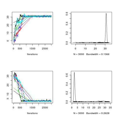
繰り返し3000回、初期値依存として捨てる数を0として、MCMC推定を実行。( chain=5 )

#fun:はサンプルを得るための関数
#theta.init:パラメータの初期値，(ここでは平均0、標準偏差30)
#burnin:初期値依存として捨てる部分である
#mcmc:サンプルを得る繰り返し回数，
#thin:サンプルを得る間隔（この例では1，すなわち毎回サンプルを得るようにしている），
#tune:はランダムウォークの大きさにかかわるパラメータ
#seed:疑似乱数のタネ
#
post1 <- MCMCmetrop1R(llnormfun, theta.init = c(0, 30), x = x, mcmc = 3000, burnin=0,seed =1)
post2 <- MCMCmetrop1R(llnormfun, theta.init = c(0, 30), x = x, mcmc = 3000, burnin=0,seed =2)
post3 <- MCMCmetrop1R(llnormfun, theta.init = c(0, 30), x = x, mcmc = 3000, burnin=0,seed =3)
post4 <- MCMCmetrop1R(llnormfun, theta.init = c(0, 30), x = x, mcmc = 3000, burnin=0,seed =4)
post5 <- MCMCmetrop1R(llnormfun, theta.init = c(0, 30), x = x, mcmc = 3000, burnin=0,seed =5)
#
geweke.diag(post1)
#|Z| > 1.96のとき危険率5%で差がある。（定常状態に達していない。）

Fraction in 1st window = 0.1
Fraction in 2nd window = 0.5

var1 var2
-2.792 18.457

posterior <- mcmc.list(post1, post2, post3, post4, post5)
#png("bayes3_1.png")
plot(posterior, trace = TRUE, density = TRUE)
#dev.off()

1	summary(posterior)

Iterations = 1:3000
Thinning interval = 1
Number of chains = 5
Sample size per chain = 3000

Empirical mean and standard deviation for each variable,
plus standard error of the mean:

Mean SD Naive SE Time-series SE
[1,] 27.648 7.722 0.06305 1.738
[2,] 7.023 9.127 0.07452 2.810
Quantiles for each variable:

2.5% 25% 50% 75% 97.5%
[1,] 2.491 30.085 30.862 31.27 32.09
[2,] 1.694 2.097 2.403 4.37 30.10

1	gelman.diag(posterior)

Potential scale reduction factors:

Point est. Upper C.I.
[1,] 1.01 1.01
[2,] 1.01 1.03

Multivariate psrf

1.01

1	effectiveSize(posterior)

var1 var2
28.46518 11.41829

1500回くらいまでは収束していない。（rstanはずっと早く収束する）

effectiveSizeも3000回＊５＝１５０００回で28 、１１

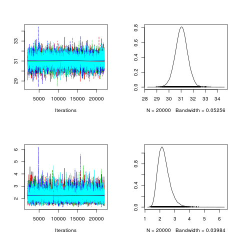
繰り返し20000回、初期値依存として捨てる数を2000として、MCMC推定を実行。( chain=5 )

lapply()関数を使ってプログラムを短く

chains  <- 1:5
seeds  <- seq(1,5,1)
posterior2  <- lapply(chains ,
			function(chain) {
				MCMCmetrop1R(fun = llnormfun ,
				theta.init = c(0,30),
				burnin = 2000,  mcmc = 20000,
				seed = seeds[chain],thin=1,
				x = x)})
#class(posterior2)
#str(posterior2)
#geweke.diag(posterior2[[1]])
post2.mcmc <- mcmc.list(posterior2)
#png("bayes3_2.png")
plot(post2.mcmc, trace = TRUE, density = TRUE)
#dev.off()

1	summary(post2.mcmc)

Iterations = 2001:22000
Thinning interval = 1
Number of chains = 5
Sample size per chain = 20000

Empirical mean and standard deviation for each variable,
plus standard error of the mean:

Mean SD Naive SE Time-series SE
[1,] 31.028 0.5133 0.001623 0.005449
[2,] 2.274 0.4033 0.001275 0.005282
Quantiles for each variable:

2.5% 25% 50% 75% 97.5%
[1,] 29.999 30.696 31.031 31.361 32.034
[2,] 1.652 1.991 2.221 2.495 3.216

1	gelman.diag(post2.mcmc)

Potential scale reduction factors:

Point est. Upper C.I.
[1,] 1 1
[2,] 1 1

Multivariate psrf

1	effectiveSize(post2.mcmc)

var1 var2
8876.217 5971.989

effectiveSize : 20000回＊5=100000回で8876, 5972

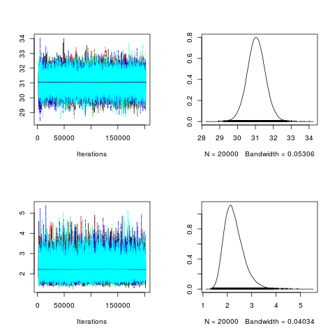
繰り返し200000回、初期値依存として捨てる数を2000、thin（サンプルを得る間隔）=10として、MCMC推定を実行。( chain=5 )

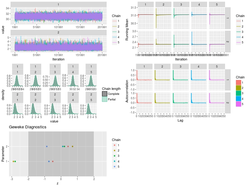
chains  <- 1:5
seeds  <- seq(1,5,1)
posterior3  <- lapply(chains ,
			function(chain) {
				MCMCmetrop1R(fun = llnormfun ,
				theta.init = c(0,30),
				burnin = 2000,  mcmc = 200000,
				seed = seeds[chain],thin=10,
				x = x)})
post3.mcmc <- mcmc.list(posterior3)
#png("bayes3_3.png")
plot(post3.mcmc, trace = TRUE, density = TRUE)
#dev.off()

1	summary(post3.mcmc)

Iterations = 2001:201991
Thinning interval = 10
Number of chains = 5
Sample size per chain = 20000

Empirical mean and standard deviation for each variable,
plus standard error of the mean:

Mean SD Naive SE Time-series SE
[1,] 31.047 0.5173 0.001636 0.001998
[2,] 2.275 0.4048 0.001280 0.001768
Quantiles for each variable:

2.5% 25% 50% 75% 97.5%
[1,] 30.028 30.71 31.045 31.38 32.078
[2,] 1.647 1.99 2.219 2.50 3.222

1	gelman.diag(post3.mcmc)

Potential scale reduction factors:

Point est. Upper C.I.
[1,] 1 1
[2,] 1 1

Multivariate psrf

1	effectiveSize(post3.mcmc)

var1 var2
67206.95 52591.34

effectiveSize : 20000回＊5=100000回で67207 , 52591

ほぼテキスト並の数値になったので以後はこの出力を使う

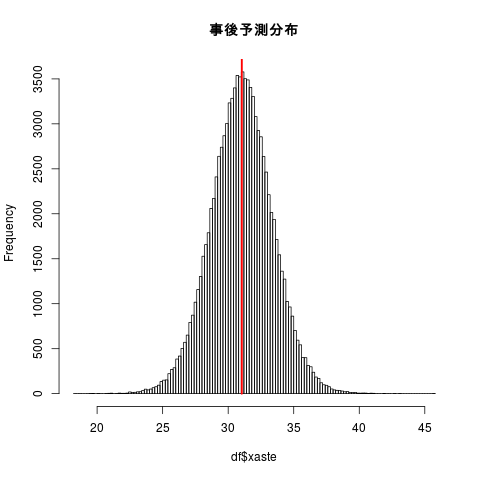
xasteは、推定されたsigma を使って正規分布から無作為に抽出する必要がある。

df <- data.frame(mu=unlist(post3.mcmc[,1]),sigma=unlist(post3.mcmc[,2]))
xaste<-rnorm(n = nrow(df), mean =df$mu, sd = df$sigma)
#
df<- data.frame(df,xaste)
#
# kanitr::kableを使って出力を工夫
#
ryou<-data.frame(c(round(mean(df[,1]),2) , round(sd(df[,1]),2) ,
	round(quantile(df[,1],c(0.025,0.05,0.5,0.95,0.975)),2)))
for (i in 2:ncol(df) ){
ryou<-cbind(ryou,data.frame(c(round(mean(df[,i]),2) , round(sd(df[,i]),2) ,
	round(quantile(df[,i],c(0.025,0.05,0.5,0.95,0.975)),2))))
}
names(ryou)<-c("mu","sigma","xaste")
rownames(ryou)<-c("EAP","post.sd","2.5%","5%","50%","95%","97.5%")
#
kable(t(ryou))

	EAP	post.sd	2.5%	5%	50%	95%	97.5%
mu	31.05	0.52	30.03	30.20	31.04	31.90	32.08
sigma	2.28	0.40	1.65	1.72	2.22	3.02	3.22
xaste	31.04	2.36	26.37	27.18	31.04	34.89	35.70

#png("bayes3_4.png")
hist(df$xaste,breaks=100,main="事後予測分布")
#abline(v=mean(df$xaste),col="red")
segments(mean(df$xaste),0,mean(df$xaste),par("usr")[4],lwd=2.5 ,col="red")
#dev.off()

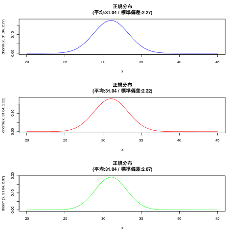
# 確率密度関数（dnorm）: 確率分布関数（pnorm）とその逆関数（qnorm）
x<-seq(20,45,0.1)
#png("bayes3_8.png")
par(mfrow=c(3,1))
curve(dnorm(x,31.04,2.27),20,45, col="blue")
title(main="正規分布\n(平均:31.04 / 標準偏差:2.27)")
curve(dnorm(x,31.04,2.22),20,45, col="red")
title(main="正規分布\n(平均:31.04 / 標準偏差:2.22)")
curve(dnorm(x,31.04,2.07),20,45, col="green")
title(main="正規分布\n(平均:31.04 / 標準偏差:2.07)")
par(mfrow=c(1,1))
#dev.off()

library(ggmcmc)
#ggmcmc(ggs(post3.mcmc), file="posterior.pdf")
#ggmcmc(ggs(post3.mcmc), plot=c("histogram", "traceplot", "geweke"))
#ggmcmc(ggs(post3.mcmc), plot=c("histogram"),file=NULL)
#ggs_histogram(ggs(post3.mcmc))
#ggs_density(ggs(post3.mcmc))
#ggs_traceplot(ggs(post3.mcmc))
#ggs_running(ggs(post3.mcmc))
#ggs_compare_partial(ggs(post3.mcmc))
#ggs_autocorrelation(ggs(post3.mcmc))
#ggs_crosscorrelation(ggs(post3.mcmc))
#ggs_Rhat(ggs(post3.mcmc)) + xlab("R_hat")
#ggs_geweke(ggs(post3.mcmc))
#
#png("bayes3_5.png",width=800,height=600)
p1<-ggs_traceplot(ggs(post3.mcmc))
p2<-ggs_running(ggs(post3.mcmc))
p3<-ggs_compare_partial(ggs(post3.mcmc))
p4<-ggs_autocorrelation(ggs(post3.mcmc))
p5<-ggs_geweke(ggs(post3.mcmc))
gridExtra::grid.arrange(p1, p2, p3, p4, p5,ncol = 2)
#dev.off()

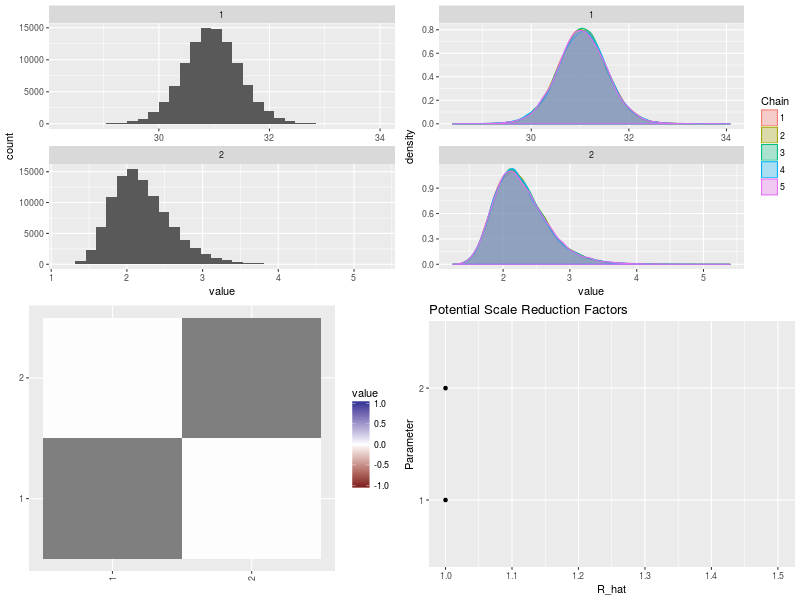
#png("bayes3_6.png",width=800,height=600)
p1<-ggs_histogram(ggs(post3.mcmc))
p2<-ggs_density(ggs(post3.mcmc))
p3<-ggs_crosscorrelation(ggs(post3.mcmc))
p4<-ggs_Rhat(ggs(post3.mcmc)) + xlab("R_hat")
gridExtra::grid.arrange(p1, p2, p3, p4,ncol = 2)
#dev.off()

p.61 生成量の推定結果

分散

1
2
3

variance <- df$sigma^2
c(EAP=round(mean(variance),3) , post.sd=round(sd(variance),3) ,
	round(quantile(variance,c(0.025,0.05,0.5,0.95,0.975)),3))

EAP post.sd 2.5% 5% 50% 95% 97.5%
5.340 2.018 2.712 2.964 4.922 9.102 10.378

変動係数

1
2
3

cv<- df$sigma/df$mu
c(EAP=round(mean(cv),3) , post.sd=round(sd(cv),3) ,
	round(quantile(cv,c(0.025,0.05,0.5,0.95,0.975)),3))

EAP post.sd 2.5% 5% 50% 95% 97.5%
0.073 0.013 0.053 0.055 0.071 0.097 0.104

効果量

c<-30
delta30<- (df$mu-c)/df$sigma
c(EAP=round(mean(delta30),3) , post.sd=round(sd(delta30),3) ,
	round(quantile(delta30,c(0.025,0.05,0.5,0.95,0.975)),3))

EAP post.sd 2.5% 5% 50% 95% 97.5%
0.474 0.237 0.012 0.085 0.473 0.865 0.939

分位点・％点

z<-qnorm(0.25, mean=0, sd=1)
qu25<- df$mu + z * df$sigma
c(EAP=round(mean(qu25),3) , post.sd=round(sd(qu25),3) ,
	round(quantile(qu25,c(0.025,0.05,0.5,0.95,0.975)),3))

EAP post.sd 2.5% 5% 50% 95% 97.5%
29.513 0.583 28.246 28.495 29.552 30.390 30.540

特定区間での観測確率

1
2
3

u29.5_30.5<-pnorm(30.5, mean =df$mu, sd = df$sigma)-pnorm(29.5, mean =df$mu, sd = df$sigma)
c(EAP=round(mean(u29.5_30.5),3) , post.sd=round(sd(u29.5_30.5),3) ,
	round(quantile(u29.5_30.5,c(0.025,0.05,0.5,0.95,0.975)),3))

EAP post.sd 2.5% 5% 50% 95% 97.5%
0.156 0.026 0.106 0.114 0.155 0.201 0.210

比の分布

c<-30
hi30<-df$xaste/c
c(EAP=round(mean(hi30),3) , post.sd=round(sd(hi30),3) ,
	round(quantile(hi30,c(0.025,0.05,0.5,0.95,0.975)),3))

EAP post.sd 2.5% 5% 50% 95% 97.5%
1.035 0.079 0.879 0.906 1.035 1.163 1.190

各種事後分布

#png("bayes3_7.png",width=800,height=600)
par(mfrow=c(2,3))
hist(variance,breaks=100,main="分散")
hist(cv,breaks=100,main="変動係数")
hist(delta30,breaks=100,main="効果量")
hist(qu25,breaks=100,main="２５％点")
hist(u29.5_30.5,breaks=100,main="U29.5 < xaste < 30.5")
hist(hi30,breaks=100,main="xaste / 30")
par(mfrow=c(1,1))
#dev.off()

研究仮説が正しい確率

30<mu

1 2	p<-table(df$mu > 30) p[2]/(p[1]+p[2])

TRUE
0.9778

29.5<mu<30.5

1 2	p<-table(df$xaste > 29.5 & df$xaste < 30.5) p[2]/(p[1]+p[2])

TRUE
0.15509

delta30 > 0.5

1 2	p<-table(delta30 > 0.5) p[2]/(p[1]+p[2])

TRUE
0.45327

29.5 < 測定値 < 30.5 の確率が20%未満の確率

1 2	p<- table(u29.5_30.5 < 0.2) p[2]/(p[1]+p[2])

TRUE
0.94793

統計ソフトRの備忘録２

心理統計法('17) その１

放送大学「心理統計法(‘17)」第3章第4章

授業ではrstanパッケージを使ってますが、MCMCpackパッケージを使ってみます。初学者ですので間違いが多々あると思います。

繰り返し3000回、初期値依存として捨てる数を0として、MCMC推定を実行。( chain=5 )

1500回くらいまでは収束していない。（rstanはずっと早く収束する）

effectiveSizeも3000回＊５＝１５０００回で28 、１１

繰り返し20000回、初期値依存として捨てる数を2000として、MCMC推定を実行。( chain=5 )

lapply()関数を使ってプログラムを短く

effectiveSize : 20000回＊5=100000回で8876, 5972

繰り返し200000回、初期値依存として捨てる数を2000、thin（サンプルを得る間隔）=10として、MCMC推定を実行。( chain=5 )

effectiveSize : 20000回＊5=100000回で67207 , 52591

ほぼテキスト並の数値になったので以後はこの出力を使う

xasteは、推定されたsigma を使って正規分布から無作為に抽出する必要がある。

p.61 生成量の推定結果

分散

変動係数

効果量

分位点・％点

特定区間での観測確率

比の分布

各種事後分布

研究仮説が正しい確率

30<mu

29.5<mu<30.5

delta30 > 0.5

29.5 < 測定値 < 30.5 の確率が20%未満の確率

本格的にやるには「rstan」でしょうけど、ベイズ統計初学者には「rstan」より「MCMCpack」の方がとっつきやすいのでは。

放送大学「心理統計法(‘17)」第3章 第4章

授業ではrstanパッケージを使ってますが、MCMCpackパッケージを使ってみます。初学者ですので間違いが多々あると思います。

繰り返し3000回、初期値依存として捨てる数を0として、MCMC推定を実行。( chain=5 )

1500回くらいまでは収束していない。（rstanはずっと早く収束する）

effectiveSizeも3000回＊５＝１５０００回で28 、 １１

繰り返し20000回、初期値依存として捨てる数を2000として、MCMC推定を実行。( chain=5 )

lapply()関数を使ってプログラムを短く

effectiveSize : 20000回＊5=100000回で8876, 5972

繰り返し200000回、初期値依存として捨てる数を2000、thin（サンプルを得る間隔）=10として、MCMC推定を実行。( chain=5 )

effectiveSize : 20000回＊5=100000回で67207 , 52591

ほぼテキスト並の数値になったので以後はこの出力を使う

xasteは、推定されたsigma を使って正規分布から無作為に抽出する必要がある。

p.61 生成量の推定結果

分散

変動係数

効果量

分位点・％点

特定区間での観測確率

比の分布

各種事後分布

研究仮説が正しい確率

30<mu

29.5<mu<30.5

delta30 > 0.5

29.5 < 測定値 < 30.5 の確率が20%未満の確率

本格的にやるには「rstan」でしょうけど、ベイズ統計初学者には「rstan」より「MCMCpack」の方がとっつきやすいのでは。

放送大学「心理統計法(‘17)」第3章第4章

effectiveSizeも3000回＊５＝１５０００回で28 、１１