Jun 24 2017

コンジョイント分析１

conjoint( tea データ) , ggplot2 , knitr , qdapTools パッケージ

conjointパッケージのデータ tea をコンジョイント分析

library(conjoint)
library(ggplot2)
library(knitr)
#install_github("trinker/qdapTools")
library(qdapTools)
#
data(tea)
#
x<-tprof
#
y<-tpref ; y<-matrix(y[,1],ncol=13,byrow=T)
#y<-as.matrix(tprefm)
#
z<-tlevn 	# level名が同じ場合(例えばyesやnoが複数ある)グラフの出力が不具合を起こす可能性有り
#
family <- gaussian
# family <- binomial
# family <- poisson
# family <- negative.binomial(3)
 kable(cor(x))

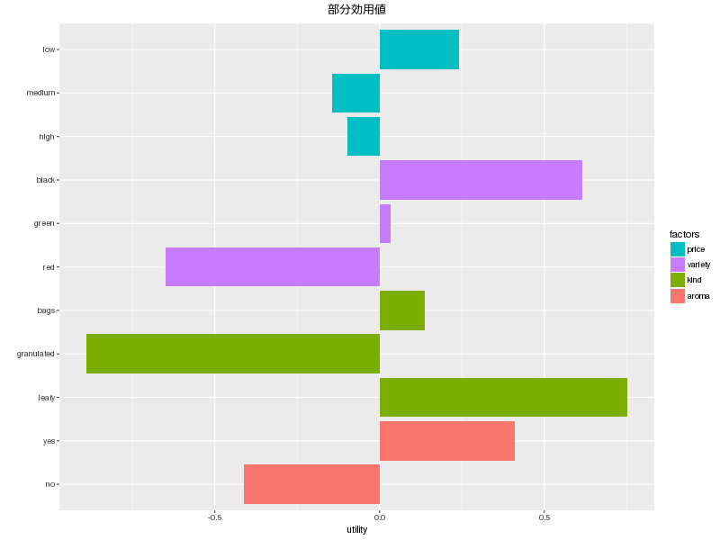
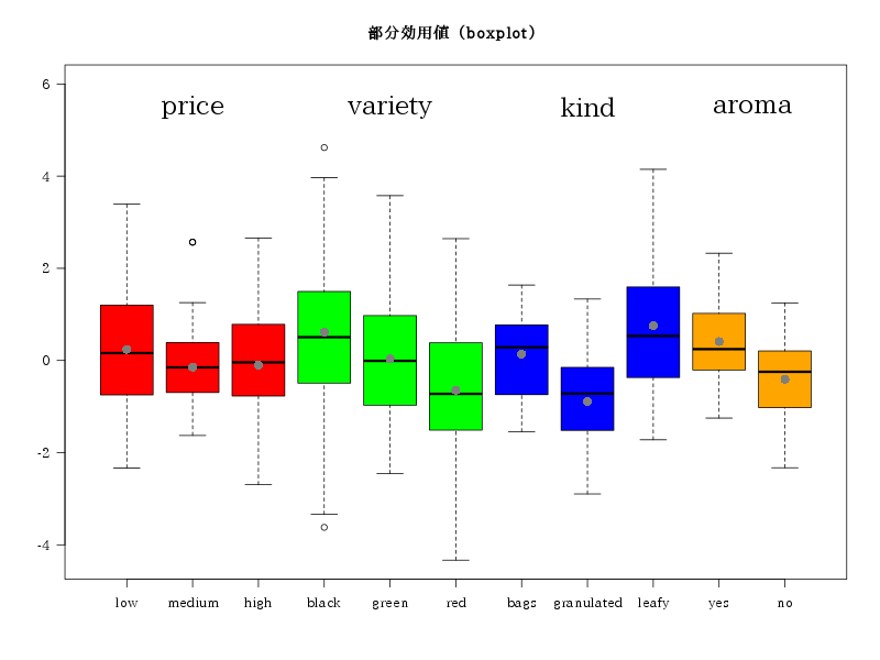
相関行列

	price	variety	kind	aroma
price	1.0000000	-0.0900000	0	-0.0474342
variety	-0.0900000	1.0000000	0	0.0474342
kind	0.0000000	0.0000000	1	0.0000000
aroma	-0.0474342	0.0474342	0	1.0000000

# 各プロファイルごとの評価点の分布の様子
#png("conj01_1.png",width=800,height=600)
par(mfrow=c(3,5))
par(family="TakaoExMincho")
for(i in 1:ncol(y)){
hist(y[,i],col="pink",main=paste0("プロファイル",i),xlab="",breaks=0:10)
}
par(mfrow=c(1,1))
#dev.off()

# 算出
#
( xnames<-colnames(x) )
( m <- length(x) ) # 4
( n <- nrow(x) ) # 13
( xnum<-as.vector(sapply(apply(x,2, unique),length)) ) #  3  3  3  2
( S <- nrow(y) ) # 100
#
# 現在のcontrastを確認。def_contrastsへ
options("contrasts")
def_contrasts<-options("contrasts")
#
# "contr.sum" : 各属性変数（因子）に含まれる（各水準に対応した）係数推定値の和がゼロになるように制約
options(contrasts = c("contr.sum", "contr.poly"))
#
mat<-NULL
U<-NULL
#
    xtmp <- paste("factor(x$", xnames, sep = "", paste(")"))
    xfrm <- paste(xtmp, collapse = "+")
    frml <- as.formula(paste("y[i,]~", xfrm))
#
for(i in 1:S ){
	glmresult<-glm( frml,family=family )
	ma<-as.matrix(glmresult$coeff)
	moma<-model.matrix(glmresult)
	U <- cbind(U,moma%*%ma)
	mat<-cbind(mat,ma)
}
#
mat<-t(mat)
#
 xx<-NULL
 for (i in 1:S){
	xx<-rbind(xx,x)
	}
  xxtmp <- paste("factor(xx$", xnames, sep = "", paste(")"))
  xxfrm <- paste(xxtmp, collapse = "+")
  glmresult<-glm(as.formula(paste("as.vector(t(y))~", xxfrm )) ,family=family  )
  print(summary(glmresult))
#
# contrastsを元に戻す。確認
options(contrasts=def_contrasts$contrasts)
options("contrasts")
#
matr<-NULL
matr<-cbind(mat[,2:xnum[1],drop=F] ,rowSums(mat[,2:xnum[1],drop=F])*(-1))
cont<-data.frame(apply(matr,1,max)-apply(matr,1,min))
#
for (i in 1 : (m-1) ){
	mat0<-cbind( mat[,(sum(xnum[1:i]) + 2 - i):(sum(xnum[1:(i + 1)]) - i),drop=F] ,
		rowSums( mat[, (sum(xnum[1:i]) + 2 - i):(sum(xnum[1:(i + 1)]) - i),drop=F])*(-1))
	cont<-cbind(cont,data.frame(apply(mat0,1,max)-apply(mat0,1,min)) )	
	matr<-cbind(matr,mat0)
	}
#
#colnames(matr)<-z[,1]
colnames(cont)<-colnames(x)
#
# cont ; matr ; U  
#
# 重要度
# 重要度得点(各要因の相対重要度の尺度)
## (計算方法)各要因の効用の範囲を、全要因の効用範囲の和で割る
## (注意)被験者ごとに別々に行われてから、全被験者の平均がとられる。
#
zyuyou<-data.frame(imp=round(apply(cont,2,mean)*100/sum(apply(cont,2,mean)) ,2) )
zyuyou$factors<-factor(rownames(zyuyou),levels=rownames(zyuyou) )
kable(zyuyou)

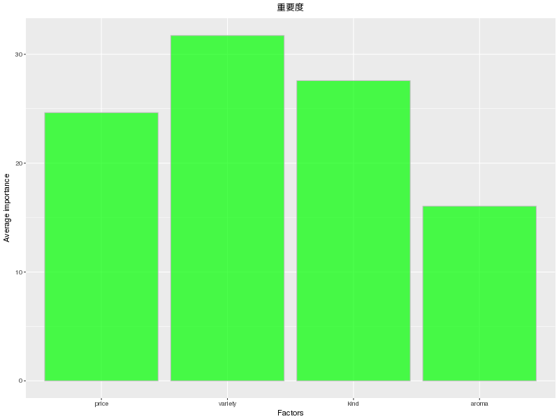
重要度得点

	imp	factors
price	24.64	price
variety	31.73	variety
kind	27.58	kind
aroma	16.05	aroma

#png("conj01_2.png",width=800,height=600)
ggplot(zyuyou,aes(x=factors,y=imp)) + 
	geom_bar(position = "dodge", stat = "identity",fill=rgb(0,1,0,0.7),colour="gray") +
	labs(x="Factors",y="Average importance",title="重要度") +
	theme(plot.title = element_text(hjust = 0.5))
#dev.off()

# 「各水準」の部分効用値
knames<-NULL
for(i in 1:length(xnames) ){
	kna <-rep(xnames[i],each=xnum[i])
	knames<-c(knames,kna)
	}
#
pl<-data.frame(factors=knames ,
	levels=factor(z[,1],levels=rev(z[,1])) , 
	utls= apply(matr,2,mean))
pl
# 切片は 
mean(mat[,1])
#
#png("conj01_3.png",width=800,height=600)
ggplot(pl,aes(x=levels,y=utls,fill=factors)) + 
	geom_bar(position = "dodge", stat = "identity") + 
	scale_fill_discrete(breaks= xnames ) +
	labs(x="",y="utility",title="部分効用値")+
	theme(plot.title = element_text(hjust = 0.5)) +
	coord_flip()
#dev.off()

#png("conj01_4.png",width=800,height=600)
par(family="TakaoExMincho")
boxplot(matr, las = 1, names = z[,1],
	col=c(rep(c("red","green","blue"),each=3),rep("orange",2)),
	ylim=c(min(matr),6))
text(2,5.5,xnames[1],cex=2)
text(5,5.5,xnames[2],cex=2)
text(8,5.5,xnames[3],cex=2)
text(10.5,5.5,xnames[4],cex=2)
title("部分効用値（boxplot）")
#lines(pl[,3],col="gray",lwd=1.5)
points(pl[,3],col="gray50",pch=16,cex=1.5)
#dev.off()

1
2
3

# クラスター分析
library(cluster)
pam(t(U),3)$clustering

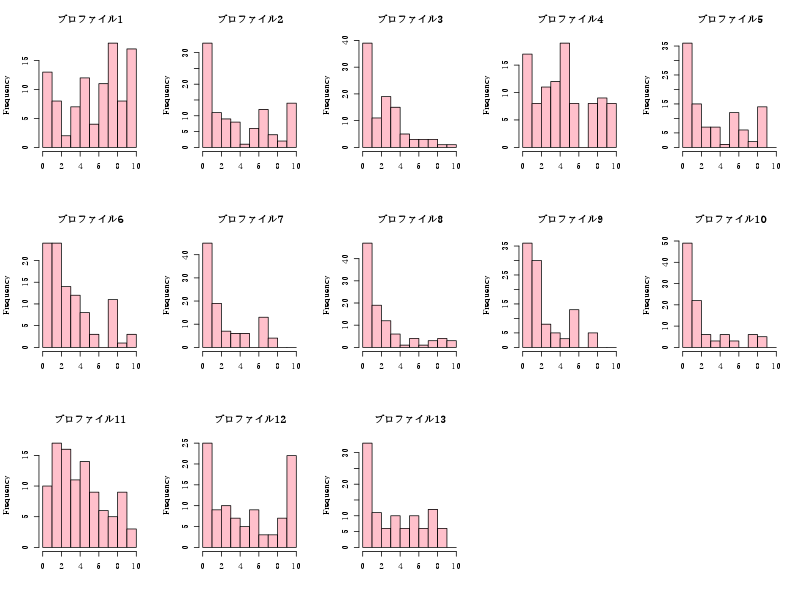
[1] 1 2 3 2 2 1 2 1 2 3 3 3 1 1 1 1 2 1 2 1 1 3 1 2 2 1 2 2 2 2 1 2 1 2 3 3 3
[38] 1 1 1 1 2 1 2 1 1 3 1 1 1 2 1 1 1 2 2 1 2 1 2 1 1 2 2 1 2 1 1 1 2 2 1 1 2
[75] 3 2 2 1 2 1 2 2 2 3 1 1 1 1 2 1 2 1 2 1 1 3 1 1 2 3

# 観測値の平均と予測値の平均の相関係数
# ピアソンの積率相関係数 r
#
cor(apply(y,2,mean),apply(U,1,mean) , method="p")  # method="p"は初期値なので必要はない
#
#[1] 0.8342373
# 順位評価の場合はこっち
# ケンドールの順位相関係数τ(tau)
# cor(apply(y,2,mean),apply(U,1,mean) , method="k")
# [1] 0.7435897

予測値の算出 (全組み合わせ)

# プロファイルの作成
# 全パターンのリスト
price<-c("low","medium","high")
variety<-c("black","green","red")
kind<-c("bags","granulated","leafy")
aroma<-c("yes","no")
#
experiment<-expand.grid(
price,
variety,
kind,
aroma )
#
# 全組み合わせは、type="full"
#
( designfull<-caFactorialDesign(data=experiment,type="full") )
#
( codefull<-caEncodedDesign(designfull) )
#
colnames(codefull) <- xnames
#
cl<-cldata <- codefull
#
for (i in 2:ncol(cl)){			# i は 2 から
	cl[,i]<-cl[,i]+sum(xnum[1:(i-1)])
	}
#
clall<-rep(0,nrow(cl))
#
for (i in 1:nrow(cl)){
	clsum<-0
	for (j in 1:ncol(cl)){
		clsum<-clsum + pl$utls[cl[i,j]]
		}
	clall[i]<-clsum	
}
#
# 切片の平均：mean(mat[,1])
cl$score<-round(clall + mean(mat[,1]),3)
#kable(data.frame(cldata,Score=cl$score))
#
# コードを水準名に変換 qdapTools::lookup
#
cldata[,1]<-lookup(cldata[,1], data.frame(1:3,price))
cldata[,2]<-lookup(cldata[,2], data.frame(1:3,variety))
cldata[,3]<-lookup(cldata[,3], data.frame(1:3,kind))
cldata[,4]<-lookup(cldata[,4], data.frame(1:2,aroma))
#
kable(data.frame(cldata,Score=cl$score))

price	variety	kind	aroma	Score
low	black	bags	yes	4.956
medium	black	bags	yes	4.573
high	black	bags	yes	4.619
low	green	bags	yes	4.376
medium	green	bags	yes	3.993
high	green	bags	yes	4.039
low	red	bags	yes	3.691
medium	red	bags	yes	3.308
high	red	bags	yes	3.354
low	black	granulated	yes	3.929
medium	black	granulated	yes	3.546
high	black	granulated	yes	3.592
low	green	granulated	yes	3.349
medium	green	granulated	yes	2.966
high	green	granulated	yes	3.012
low	red	granulated	yes	2.665
medium	red	granulated	yes	2.281
high	red	granulated	yes	2.327
low	black	leafy	yes	5.572
medium	black	leafy	yes	5.189
high	black	leafy	yes	5.235
low	green	leafy	yes	4.992
medium	green	leafy	yes	4.609
high	green	leafy	yes	4.655
low	red	leafy	yes	4.307
medium	red	leafy	yes	3.924
high	red	leafy	yes	3.970
low	black	bags	no	4.135
medium	black	bags	no	3.751
high	black	bags	no	3.797
low	green	bags	no	3.555
medium	green	bags	no	3.171
high	green	bags	no	3.217
low	red	bags	no	2.870
medium	red	bags	no	2.487
high	red	bags	no	2.533
low	black	granulated	no	3.108
medium	black	granulated	no	2.725
high	black	granulated	no	2.771
low	green	granulated	no	2.528
medium	green	granulated	no	2.145
high	green	granulated	no	2.191
low	red	granulated	no	1.843
medium	red	granulated	no	1.460
high	red	granulated	no	1.506
low	black	leafy	no	4.751
medium	black	leafy	no	4.367
high	black	leafy	no	4.413
low	green	leafy	no	4.171
medium	green	leafy	no	3.787
high	green	leafy	no	3.833
low	red	leafy	no	3.486
medium	red	leafy	no	3.103
high	red	leafy	no	3.149

シミュレーションの選好確率(各シミュレーションケースが最も好ましいものとして選択される確率)

conjoint package の tea data の tsimp

simp <- simpdata <- tsimp
#
# simpの値とz[,1]の順序を対応させる
for (i in 2:ncol(simp)){
	simp[,i]<-simp[,i]+sum(xnum[1:(i-1)])
	}
simp ; z[,1]
#
#   price variety kind aroma
# 1     3       5    8    11
# 2     1       6    7    10
# 3     2       6    9    11
# 4     3       4    8    10
#
# [1] low        medium     high       black      green      red       
# [7] bags       granulated leafy      yes        no        
#
simpF<-NULL
#
for (i in 1:S){
	simpsum<-rep(0,nrow(simp))
	for (j in 1:ncol(simp)){
		for (k in 1:nrow(simp)){
		simpsum[k]<- simpsum[k] + matr[i,simp[k,j]]
		}
	}
	# 正規化(最小値 0、最大値 1)
	simpsum<-scale(simpsum, center = min(simpsum), scale = (max(simpsum) -min(simpsum)))[,1]
	simpF<-rbind(simpF,t( simpsum))
}
#
## 最大効用値モデル 最大のものが確率１,ほかのすべてのものが確率０
MaxModel <- colSums(simpF == 1) * 100 /sum(simpF == 1)    # 列ごとに値１ の数を数えて総数で割る
( MaxModel <- round(MaxModel ,2) )
#
## BTL (Bradley-Terry-Luce) モデル  効用の割合が確率
BTLModel<- colSums(simpF) * 100 / sum(simpF) # 列ごとの合計 / 総合計
( BTLModel <- round(BTLModel ,2) )
#
## ロジット モデル  効用を指数に変換して、その割合が確率
LogitModel <- colSums(exp(simpF)) * 100/ sum(exp(simpF))   # 効用を指数に変換 -> 列ごとの合計 / 総合計
( LogitModel <- round(LogitModel ,2) )
#
#kable(data.frame(simpdata,MaxModel,BTLModel,LogitModel))
#
# コードを水準名に変換 qdapTools::lookup
#
simpdata[,1]<-lookup(simpdata[,1], data.frame(1:3,price))
simpdata[,2]<-lookup(simpdata[,2], data.frame(1:3,variety))
simpdata[,3]<-lookup(simpdata[,3], data.frame(1:3,kind))
simpdata[,4]<-lookup(simpdata[,4], data.frame(1:2,aroma))
#
kable(data.frame(simpdata,MaxModel,BTLModel,LogitModel))

price	variety	kind	aroma	MaxModel	BTLModel	LogitModel
high	green	granulated	no	11	14.11	19.99
low	red	bags	yes	28	30.77	27.60
medium	red	leafy	no	26	25.74	25.30
high	black	granulated	yes	35	29.39	27.12

conjoint パッケージとは最大効用値モデル以外は結果が一致しない!!!

1	ShowAllSimulations(tsimp, tpref, tprof)

TotalUtility MaxUtility BTLmodel LogitModel
1 2,19 11 18,85 13,04
2 3,69 28 28,96 34,84
3 3,10 26 30,14 35,79
4 3,59 35 22,06 16,33

シミュレーションの選好確率(全組み合わせ)

予測値の算出 (全組み合わせ)で作成した codefullを使う

simp <- simpdata <- codefull
#
# simpの値とz[,1]の順序を対応させる
for (i in 2:ncol(simp)){
	simp[,i]<-simp[,i]+sum(xnum[1:(i-1)])
	}
#
simpF<-NULL
#
for (i in 1:S){
	simpsum<-rep(0,nrow(simp))
	for (j in 1:ncol(simp)){
		for (k in 1:nrow(simp)){
		simpsum[k]<- simpsum[k] + matr[i,simp[k,j]]
		}
	}
	# 正規化(最小値 0、最大値 1)
	simpsum<-scale(simpsum, center = min(simpsum), scale = (max(simpsum) -min(simpsum)))[,1]
	simpF<-rbind(simpF,t( simpsum))
}
#
## 最大効用値モデル 最大のものが確率１,ほかのすべてのものが確率０
MaxModel <- colSums(simpF == 1) * 100 /sum(simpF == 1)    # 列ごとに値１ の数を数えて総数で割る
( MaxModel <- round(MaxModel ,2) )
#
## BTL (Bradley-Terry-Luce) モデル  効用の割合が確率
BTLModel<- colSums(simpF) * 100 / sum(simpF) # 列ごとの合計 / 総合計
( BTLModel <- round(BTLModel ,2) )
#
## ロジット モデル  効用を指数に変換して、その割合が確率
LogitModel <- colSums(exp(simpF)) * 100/ sum(exp(simpF))   # 効用を指数に変換 -> 列ごとの合計 / 総合計
( LogitModel <- round(LogitModel ,2) )
#
#kable(data.frame(simpdata,MaxModel,BTLModel,LogitModel))
#
# コードを水準名に変換 qdapTools::lookup
#
simpdata[,1]<-lookup(simpdata[,1], data.frame(1:3,price))
simpdata[,2]<-lookup(simpdata[,2], data.frame(1:3,variety))
simpdata[,3]<-lookup(simpdata[,3], data.frame(1:3,kind))
simpdata[,4]<-lookup(simpdata[,4], data.frame(1:2,aroma))
#
kable(data.frame(simpdata,MaxModel,BTLModel,LogitModel))

price	variety	kind	aroma	MaxModel	BTLModel	LogitModel
low	black	bags	yes	7.55	2.39	2.13
medium	black	bags	yes	2.83	2.31	2.06
high	black	bags	yes	8.49	2.31	2.09
low	green	bags	yes	5.66	2.10	1.97
medium	green	bags	yes	0.00	2.02	1.90
high	green	bags	yes	0.00	2.01	1.91
low	red	bags	yes	0.00	1.87	1.85
medium	red	bags	yes	0.00	1.79	1.79
high	red	bags	yes	0.94	1.78	1.81
low	black	granulated	yes	0.00	2.00	1.91
medium	black	granulated	yes	0.00	1.92	1.87
high	black	granulated	yes	0.00	1.92	1.88
low	green	granulated	yes	0.00	1.71	1.77
medium	green	granulated	yes	2.83	1.62	1.73
high	green	granulated	yes	0.00	1.62	1.73
low	red	granulated	yes	0.00	1.48	1.66
medium	red	granulated	yes	0.94	1.39	1.62
high	red	granulated	yes	0.00	1.39	1.63
low	black	leafy	yes	11.32	2.67	2.27
medium	black	leafy	yes	0.94	2.59	2.21
high	black	leafy	yes	2.83	2.58	2.23
low	green	leafy	yes	9.43	2.37	2.13
medium	green	leafy	yes	0.00	2.29	2.06
high	green	leafy	yes	3.77	2.29	2.08
low	red	leafy	yes	0.00	2.14	1.99
medium	red	leafy	yes	2.83	2.06	1.94
high	red	leafy	yes	7.55	2.06	1.95
low	black	bags	no	0.00	2.05	1.94
medium	black	bags	no	0.00	1.97	1.89
high	black	bags	no	4.72	1.96	1.89
low	green	bags	no	3.77	1.75	1.80
medium	green	bags	no	0.00	1.67	1.74
high	green	bags	no	0.00	1.67	1.73
low	red	bags	no	3.77	1.52	1.70
medium	red	bags	no	2.83	1.44	1.66
high	red	bags	no	0.00	1.44	1.65
low	black	granulated	no	0.00	1.66	1.75
medium	black	granulated	no	0.00	1.58	1.72
high	black	granulated	no	0.94	1.57	1.71
low	green	granulated	no	0.00	1.36	1.63
medium	green	granulated	no	0.00	1.28	1.60
high	green	granulated	no	0.94	1.28	1.58
low	red	granulated	no	0.00	1.13	1.53
medium	red	granulated	no	0.00	1.05	1.51
high	red	granulated	no	0.00	1.05	1.49
low	black	leafy	no	1.89	2.32	2.07
medium	black	leafy	no	6.60	2.24	2.03
high	black	leafy	no	0.00	2.24	2.02
low	green	leafy	no	1.89	2.02	1.95
medium	green	leafy	no	0.94	1.94	1.90
high	green	leafy	no	0.00	1.94	1.89
low	red	leafy	no	0.00	1.79	1.82
medium	red	leafy	no	2.83	1.71	1.79
high	red	leafy	no	0.94	1.71	1.78

MaxModel が整数ではない？

1	sum(simpF == 1)

[1] 106

同点が６個ある。