Jan 8 2017

日銀買入額(2010-12-15～2017-01-07)

ggplot2,xts,Quandl,gdata パッケージ

(過去の記事)
日銀買入額
 日銀買入額(2010-12-15～2015-07-09)
日銀買入額(2010-12-15～2016-02-19)
日銀買入額(2010-12-15～2016-06-10)

(使用したデータ)

(作成したデータファイル)
データファイル:2010_2016 (コードの中で読み込む)
d2010_2016.RData

2016年4月以降の買入結果は、ETF (1) 右記以外 (2) 設備投資および人材投資に積極的に取り組んでいる企業を支援するためのETFに分かれている。

library(gdata)
#http://www3.boj.or.jp/market/jp/pastetfreit.zip 解凍
d201601_03 <- read.xls("2016 (Purchases until March).xls",header=F,skip=8)
d201604_12 <- read.xls("2016 (Purchases from April).xls",header=F,skip=7)
load(url("http://statrstart.github.io/data/d2010_2015.RData"))
#
head(d2010_2015);tail(d2010_2015)
head(d201601_03);tail(d201601_03)
head(d201604_12);tail(d201604_12)
#
#2016年3月以前の買入結果に変数ETF2を加える
d2010_2016<-data.frame(date=d2010_2015[,1],ETF=d2010_2015[,2],ETF2=rep(NA,nrow(d2010_2015)),REIT=d2010_2015[,3])
head(d2010_2016) ; tail(d2010_2016)
d<-data.frame(date=d201601_03[,2],ETF=d201601_03[,3],ETF2=rep(NA,nrow(d201601_03)),REIT=d201601_03[,4])
d2010_2016<-rbind(d2010_2016,d)
#
d201604_12<-d201604_12[,2:5]
names(d201604_12)<-c("date","ETF","ETF2","REIT")
d2010_2016<-rbind(d2010_2016,d201604_12)
#
#nrow(d2010_2016)
#nrow(unique(d2010_2016))
# NAを0に置き換え
d2010_2016$ETF[is.na(d2010_2016$ETF)]<-0
d2010_2016$ETF2[is.na(d2010_2016$ETF2)]<-0
d2010_2016$REIT[is.na(d2010_2016$REIT)]<-0
#
#save("d2010_2016", file="d2010_2016.RData")

(コードの中で読み込むデータ:2017年分)
2017年の買入結果

library(xts)
library(gdata)
library(ggplot2)
library(grid) 
library(Quandl)
#
#作成したデータファイル読み込み
#load("d2010_2016.RData")
load(url("http://statrstart.github.io/data/d2010_2016.RData"))
#
#日銀のサイトからデータを取り込む
#2017年3月以前の買入結果
temp <- tempfile()
#download.file("http://www3.boj.or.jp/market/jp/pastetfreit.zip",temp)
download.file("http://www3.boj.or.jp/market/jp/etfreit.zip",temp)
con <- unzip(temp, "2017.xls")
d201701_03 <- read.xls(con,header=F,skip=7)
unlink(temp)
#2017年4月以降の買入結果
#temp <- tempfile()
#download.file("http://www3.boj.or.jp/market/jp/etfreit.zip",temp)
#con <- unzip(temp, "2017.xls")
#d201704 <- read.xls(con,header=F,skip=7)
#unlink(temp)
#
#d2017<-rbind(d201701_03[,2:5],d201604[,2:5]) 
d2017<-d201701_03[,2:5]
names(d2017)<-c("date","ETF","ETF2","REIT")
#
d2017$ETF[is.na(d2017$ETF)]<-0
d2017$ETF2[is.na(d2017$ETF2)]<-0
d2017$REIT[is.na(d2017$REIT)]<-0
#
head(d2017) ; tail(d2017)
#rbind
d2010_2017<-rbind(d2010_2016,d2017)
#
x <- read.zoo(d2010_2017)
#
#ETF累計
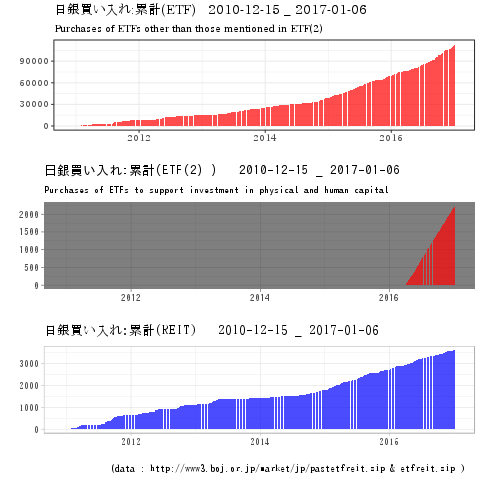
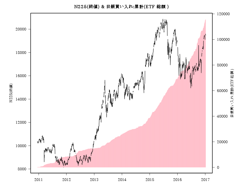
a1<-ggplot(data = fortify(cumsum(x[,1]), melt = TRUE),aes(x = Index, y = Value) ) +
geom_bar(stat="identity",position=position_dodge(),fill=rgb(1,0,0,alpha=0.7)) +
labs(title=paste("日銀買い入れ:累計(ETF)  ",d2010_2017[1,"date"],"_",d2010_2017[nrow(d2010_2017),"date"]),
    subtitle = "Purchases of ETFs other than those mentioned in ETF(2)", x="", y="")
a1<-a1 + theme_bw(base_size = 11, base_family = "IPAPMincho")
#
a2<-ggplot(data = fortify(cumsum(x[,2]), melt = TRUE),aes(x = Index, y = Value) ) +
geom_bar(stat="identity",position=position_dodge(),fill=rgb(1,0,0,alpha=0.7)) +
labs(title=paste("日銀買い入れ:累計(ETF(2) )  ",d2010_2017[1,"date"],"_",d2010_2017[nrow(d2010_2017),"date"]), 
    subtitle = "Purchases of ETFs to support investment in physical and human capital",x="", y="")
a2<-a2 + theme_dark(base_size = 11, base_family = "IPAGothic")
#REIT累計
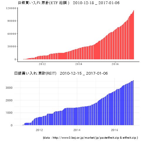
b<-ggplot(data = fortify(cumsum(x[,3]), melt = TRUE),aes(x = Index, y = Value) ) +
geom_bar(stat="identity",position=position_dodge(),fill=rgb(0,0,1,alpha=0.7)) +
labs(title=paste("日銀買い入れ:累計(REIT)  ",d2010_2017[1,"date"],"_",d2010_2017[nrow(d2010_2017),"date"]), 
     caption = "(data : http://www3.boj.or.jp/market/jp/pastetfreit.zip & etfreit.zip )  ",x="", y="")
b<-b + theme_light(base_size = 11, base_family = "TakaoMincho")
#png("boj20170106.png")
grid.newpage() #空の画面を作る
pushViewport(viewport(layout=grid.layout(3, 1))) #画面を区切る
print(a1, vp=viewport(layout.pos.row=1)) 
print(a2, vp=viewport(layout.pos.row=2)) 
print(b, vp=viewport(layout.pos.row=3)) 
#dev.off()

#ETF累計(ETFとETF2の合計)
x1<-x[,1]+x[,2]
a<-ggplot(data = fortify(cumsum(x1[,1]), melt = TRUE),aes(x = Index, y = Value) ) +
geom_bar(stat="identity",position=position_dodge(),fill=rgb(1,0,0,alpha=0.7)) +
labs(title=paste("日銀買い入れ:累計(ETF 総額 )  ",d2010_2017[1,"date"],"_",d2010_2017[nrow(d2010_2017),"date"]), 
    x="", y="")
a<-a + theme_classic(base_size = 11, base_family = "TakaoPMincho")
#
b<-ggplot(data = fortify(cumsum(x[,3]), melt = TRUE),aes(x = Index, y = Value) ) +
geom_bar(stat="identity",position=position_dodge(),fill=rgb(0,0,1,alpha=0.7)) +
labs(title=paste("日銀買い入れ:累計(REIT)  ",d2010_2017[1,"date"],"_",d2010_2017[nrow(d2010_2017),"date"]), 
    caption = "(data : http://www3.boj.or.jp/market/jp/pastetfreit.zip & etfreit.zip )  ",x="", y="")
b<-b + theme_minimal(base_size = 11, base_family = "TakaoExGothic")
#png("boj20170106_2.png")
grid.newpage() #空の画面を作る
pushViewport(viewport(layout=grid.layout(2, 1))) #画面を区切る
print(a, vp=viewport(layout.pos.row=1)) 
print(b, vp=viewport(layout.pos.row=2)) 
#dev.off()

#日経平均株価
N225=Quandl("YAHOO/INDEX_N225", collapse="daily", start_date="2010-12-15", type="xts")
#買入日の株価指数の終値でETF(日経平均株価)の買入を行ったと仮定する
dat<-merge(d2010_2017,data.frame(date=index(N225),coredata(N225[,"Close"])))
#
( sum(dat$ETF) + sum(dat$ETF2))/sum(dat$ETF/dat$Close)

15541.79

#png("boj20170106_03.png",width=800,height=640)
par(mar=c(5,7, 3,7))  
par(family="TakaoPMincho")
plot.zoo(merge(N225[,"Close"],cumsum(x1[,1]))[,2],type="h",lend=1,col="pink",xlab="",ylab="",yaxt = "n")
# 右の縦軸のラベル
mtext("日銀買い入れ:累計(ETF 総額 )",side = 4, line =4)  
# 右の縦軸を表示
axis(4,las=1)
par(new=T)
plot.zoo(merge(N225[,"Close"],cumsum(x1[,1]))[,1],xlab="",ylab="",xaxt = "n",las=1,lwd=1.5)
mtext("N225(終値)",side = 2, line = 4) 
title("N225(終値) & 日銀買い入れ:累計(ETF 総額 )")
#dev.off()

#png("boj20170106_04.png",width=800,height=640)
xx<-merge(N225[,"Close"],cumsum(x1[,1]))
par(mar=c(5,7, 3,7))  
par(family="TakaoPMincho")
plot.zoo(xx[,2],type="h",lend=1,col="pink",xlab="",ylab="",yaxt = "n")
# 右の縦軸のラベル
mtext("日銀買い入れ:累計(ETF 総額 )",side = 4, line =4)  
# 右の縦軸を表示
#axis(4,las=1)
axis(4,at=seq(0,120000,20000),labels=c(0,paste0(seq(2,12,2),"兆円")),las=1 )                      
par(new=T)
plot.zoo(xx[,1],xlab="",ylab="",xaxt = "n",las=1,lwd=1.5)
mtext("N225(終値)",side = 2, line = 4) 
title("N225(終値) & 日銀買い入れ:累計(ETF 総額 )")
#dev.off()