ggplot2,quantmod , cowplot パッケージ 他
増減率の計算式に間違いがありました。
次の記事「GPIFの運用(2015年度)(その2)」では説明変数を変更しました。
(参考)
年金、5兆円損失の見通し 運用法人、株積極投資が裏目に
(GPIFの運用に詳しい専門家の試算)
二〇一五年度、独立行政法人「GPIF」が約五兆一千億円の損失
内訳
- 外国株式:三兆六千億円の損失
- 国内株:三兆五千億円の損失
- 外国債券:五千億円の損失
- 国債など国内債券:二兆六千億円の利益
GPIFの評価損は5.5兆円か、参院選後に公表先送りとの見方も - 昨年度の運用で5.5兆円前後の評価損を被ったもよう
- 日銀がマイナス金利の導入を発表した29日を境として、基準価額が大きく上昇
自分なりに試算してみた
(注意)GPIFのデータはサイトのpdfを見て手入力したので間違いがあるかもしれません。
(データ)
運用状況
バックナンバー(運用状況)
GPIFのデータ
|
|
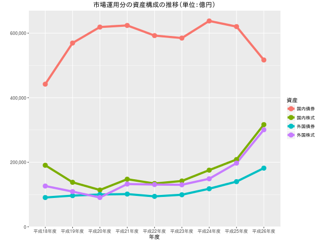
GPIFのデータをプロット
|
|
|
|
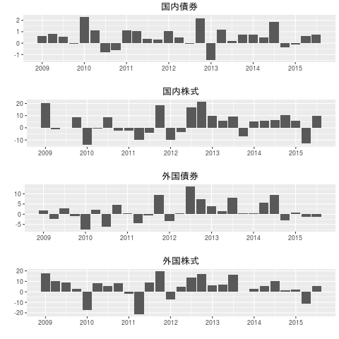
増減率の上限下限を4つとも等しくした。
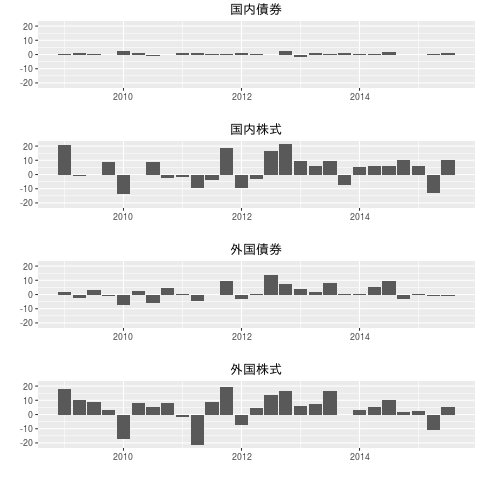
- 国内債券の増減率の振れ幅が他に比べてかなり小さいことが分かる。
GPIFの運用資産のベンチマーク
国内株式
- TOPIX(配当込み)
外国株式
- MSCI KOKUSAI(円ベース、配当込み、管理運用法人の配当課税要因考慮後)、
- MSCI EMERGING MARKETS( 円ベース、配当込み、税引き後)
- MSCI ACWI(除く日本、円ベース、配当込み、管理運用法人の配当課税要因考慮後)の複合インデックス
(試算に用いたデータ)
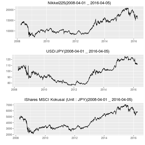
国内株式、外国株式については Yahoo Finance(com)から入手できる(quantmod::getSymbols 関数を使用)
-「Nikkei225」
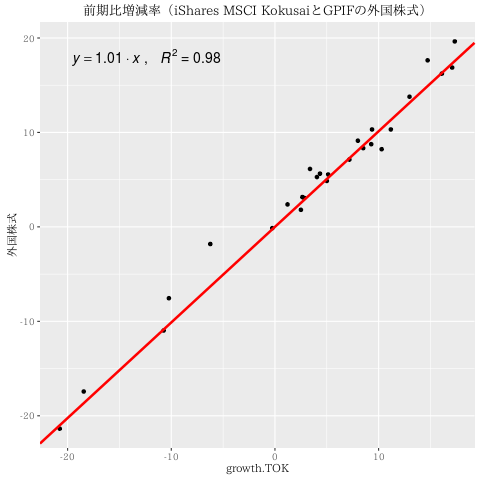
-「iShares MSCI Kokusai (TOK) に USD/JPY をかけて円ベースにしたもの」で代用
国内債券
- NOMURA-BPI「除くABS」
- NOMURA-BPI国債
- NOMURA-BPI/GPIF Customizedの複合インデックス
外国債券
- シティ世界国債インデックス(除く日本、ヘッジなし・円ベース。以下同じ。)
- 世界BIG債券インデックス(除く日本円、ヘッジなし・円ベース。以下同じ。)の複合インデックス
(試算に用いたデータ)
国内債券、外国債券については「モーニングスターのサイト」からダウンロードしたデータを使います。
SMT 国内債券インデックス・オープンの基準価額
2008/4/1 から 2015/3/31 月末ベース
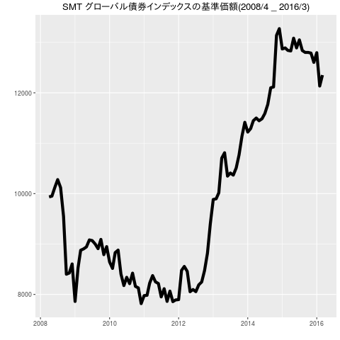
SMT グローバル債券インデックス
2008/4/1 から 2015/3/31 月末ベース
国内株式、外国株式の試算に用いるデータをダウンロード、プロット
|
|
平成27年度のGPIFの損益額を試算する。
平成27年度第4四半期の各資産の損益率を計算する。
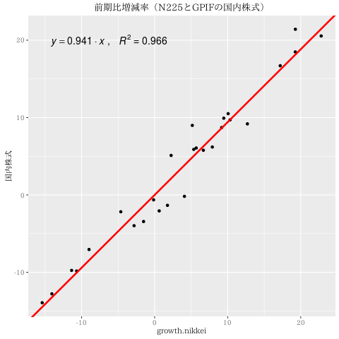
国内株式
|
|
説明変数(N225データ)の増減率が0のときには目的変数(GPIFの国内株式)の増減率も0とします。(切片0)
(理由)
切片がマイナスだとすると、説明変数の増減率がずーーーっと0だとしても、目的変数の増減率がずーーーっとマイナス。
国内株式の額が下がりつづけることになる。切片がプラスの場合は国内株式の額が上がりつづけることになる。
|
|
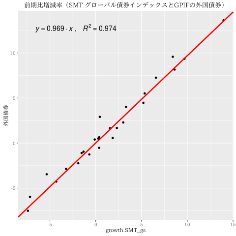
N225の増減率とGPIFの国内株式の増減率の関係を視覚化
(参考)
ggplot2: Adding Regression Line Equation and R2 on graph
|
|
(グラフは省略)
cowplot パッケージを使います。
|
|
|
|
外国株式
|
|
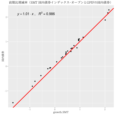
国内債券
|
|
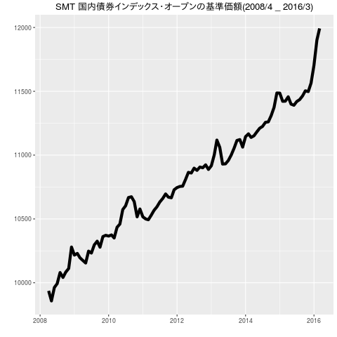
- 日銀のマイナス金利の導入によって基準価額が大きく上昇したのがわかります。(でも、上がったものは必ず下がる!)
|
|
外国債券
|
|
|
|
|
|
試算
(試算1) 平成27年度(2015)には資産の売買をしていないと仮定する
|
|
約4兆3503億円の損失
(試算2) 平成27年度(2015)第4四半期には資産の売買をしていないと仮定する
第1四半期から第3四半期までの増減額は公表済み
運用資産額(平成27年度第3四半期末現在)
1398249
運用資産別の構成割合(年金積立金全体)
国内債券 37.76% 527979(=139824937.76/100)
国内株式 23.35% 326491(=139824923.35/100)
外国債券 13.50% 188764(=139824913.50/100)
外国株式 22.82% 319080(=139824922.82/100)
資産全体の増減額は第1四半期から第3四半期までの増減額に第4四半期の増減額を加えればよい
|
|
約4兆7273億円の損失
資産別収益率(四半期別)の状況 (2015年度第4四半期(推定を含む))
|
|
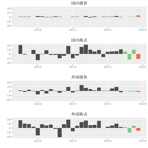
- palegreen:2015年度第1から第4四半期
- tomato:2015年度第4四半期(推定)