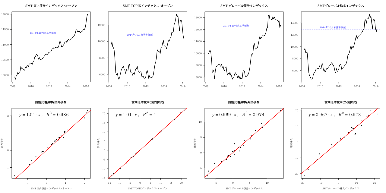
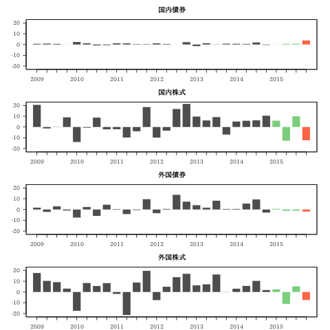
GPIFの運用(2015年度)(その2)

XML ,xts パッケージ 他

前の記事 : GPIFの運用

説明変数に使う投信の月次データをyahoo ファイナンス Japan から取り込む。
説明変数に使う投信

  1. SMT 国内債券インデックス・オープン
  2. SMT TOPIXインデックス・オープン
  3. SMT グローバル債券インデックス
  4. SMTグローバル株式インデックス”
    説明変数に使うデータを変更することによって国内株式の決定係数は上昇。外国株式は微減。
    国内債券,外国債券は同じデータなので変わらず。国内債券 : 0.986、外国債券 : 0.974
    国内株式 : 0.966 -> 1
    外国株式 : 0.98 -> 0.973

今回はggplot2 パッケージは使いません。

1
2
3
4
5
6
7
8
9
10
11
12
13
14
15
16
17
18
19
20
21
22
23
24
25
26
27
library(XML)
library(xts)
#
#### GPIFのデータ
#
#市場運用分の資産構成の推移(単位:億円)
GPIF<-data.frame(
年度=c("平成18年度","平成19年度","平成20年度","平成21年度","平成22年度","平成23年度","平成24年度","平成25年度","平成26年度"),
国内債券=c(441997,569443,618887,623923,592522,584785,637830,620364,516915),
国内株式=c(190676,137923,113986,147497,134154,141992,175575,208466,316704),
外国債券=c(90694,96641,100135,101449,94283,99301,117896,139961,181815),
外国株式=c(126376,109057,90781,132523,130919,130205,148758,197326,300772)
)
#
#png("GPIF003.png",width=640)
options(scipen=10)
par(mar=c(4,5,3,8),family = "TakaoExMincho",xpd=T)
#yaxs="i"で0から下のブランクをなくす。
matplot(1:nrow(GPIF),GPIF[,-1],type="o",pch=20,lwd=2,cex=2,xaxt = "n",yaxt = "n",col=1:4,lty=1,xlab="",ylab="",ylim=c(0,max(GPIF[,2:4])*1.05),yaxs="i")
axis(1,1:nrow(GPIF),labels=GPIF[,1])
#コンマで3桁ごとに区切る
Y=seq(0,600000,100000)
axis(2, Y, labels = prettyNum(Y, big.mark = ","),las=1)
legend(par("usr")[2]*1.01,par("usr")[3]*0.2+par("usr")[4]*0.8,legend=colnames(GPIF[,-1]),pch=20,lty=1,col=1:4,bty="n",,title="資産")
title("市場運用分の資産構成の推移(単位:億円)")
par(xpd=F)
#dev.off()

1
2
3
4
5
6
7
8
#資産別収益率(四半期別)の状況
#2009年第1四半期から2015年第3四半期まで
国内債券<-c(0.62,0.84,0.58,-0.07,2.29,1.1,-0.81,-0.61,1.11,1.06,0.38,0.34,1.04,0.49,-0.06,2.17,-1.48,1.18,0.18,0.74,0.72,0.53,1.88,-0.38,-0.1,0.6,0.75)
国内株式<-c(20.55,-1.34,-0.18,8.99,-13.93,-0.63,8.71,-2.17,-2.06,-9.75,-3.97,18.49,-9.83,-3.43,16.71,21.42,9.7,6.07,9.19,-7.05,5.11,5.78,6.2,10.51,5.89,-12.78,9.92)
外国債券<-c(1.68,-2.24,2.91,-0.95,-7.51,2.29,-5.97,4.47,0.4,-4.27,-0.53,9.58,-3.46,0.56,13.62,7.26,4.01,1.64,8.16,0.51,0.55,5.51,9.36,-2.86,0.65,-1.26,-1.1)
外国株式<-c(17.64,10.32,9.13,3.16,-17.43,8.34,5.55,8.23,-1.81,-21.36,8.76,19.64,-7.55,4.87,13.78,16.87,6.14,7.13,16.23,-0.13,3.06,5.64,10.32,1.81,2.38,-10.97,5.28)
GPIF2<-data.frame(国内債券,国内株式,外国債券,外国株式)
gp<-as.xts(ts(GPIF2,start=c(2009,1),freq=4))

説明変数に使う投信の月次データをyahoo ファイナンス Japan から取り込む。

1
2
3
4
5
6
7
8
9
10
11
12
13
14
15
16
17
18
19
20
21
22
23
24
25
26
27
28
29
30
31
32
33
34
35
36
37
38
39
40
41
42
43
44
45
46
47
48
49
50
51
52
53
54
55
56
57
58
59
60
61
62
63
64
65
66
67
68
69
70
71
72
73
74
75
76
77
from.year<-2008
#from.monthは 4 にする。四半期データに変換するため。(始まりは4月)
from.month<-4
to.year<-2016
to.month<-3
#
assets<-c("国内債券","国内株式","外国債券","外国株式")
#説明変数として用いるファンド名(これより当てはまりのよい投信が見つかったら変更)
fundname<-c("SMT 国内債券インデックス・オープン","SMT TOPIXインデックス・オープン","SMT グローバル債券インデックス","SMTグローバル株式インデックス")
#ファンドのコード(これより当てはまりのよい投信が見つかったら変更)
explanatory<-c(64315081,64313081,64316081,64314081)
#
#png("GPIF001.png",width=1280,height=640)
#linux
par(mfcol=c(2,4),family = "TakaoExMincho")
#windows
#windowsFonts(MIN = windowsFont("MS Mincho"))
#par(mfcol=c(2,4),family = "MIN")
#算出した増減率を入れるベクトル
zougen<-rep(NA,4)
#
for (i in 1:4){
data<-read.table(text = "",col.names =c("date","NAV"))
num<-ceiling((12*(to.year-from.year)+(to.month-from.month+1))/20)
for (j in 1:num){
read2 <-
readHTMLTable(paste0("http://info.finance.yahoo.co.jp/history/?code=",explanatory[i],"&sy=",from.year,"&sm=",from.month,"&ey=",to.year,"&em=",to.month,"&tm=m&p=",j))
#
temp<- data.frame(date=paste0(gsub("月","",chartr("年","-",read2[[2]][,1])),"-01"),
NAV=as.numeric(gsub(",","",read2[[2]][,2])))
data<-rbind(data,temp)
}
names(data)<-c("date",assets[i])
x<-coredata(xts(read.zoo(data))[,1])
if (i==1) {
funddata<-as.xts(read.zoo(data))
names(funddata)<-assets[i]
} else {
fundtemp<-as.xts(read.zoo(data)) ; names(fundtemp)<-assets[i]
funddata<-merge(funddata,fundtemp)
}
#
plot(ts(x,start=c(from.year,from.month),freq=12),lwd=2,xlab="",ylab="",las=1)
#構成割合の目標値の変更が行われた2014年10月31日の指数水準を青の破線で示す。
abline(h=coredata(xts(read.zoo(data))["2014-10"]),col="blue",lty=2)
text(par("usr")[1] * 0.6 + par("usr")[2]*0.4 ,coredata(xts(read.zoo(data))["2014-10"]),"2014年10月末基準価額",pos=3,col="blue")
title(fundname[i])
#title(paste0(fundname[i],"(",from.year,"/",from.month,"~",to.year,"/",to.month,")"))
#
index.quarterlast<-endpoints(as.xts(ts(x,start=c(from.year,from.month),freq=12)),on="quarters")
SMT<-ts(coredata(as.xts(ts(x,start=c(from.year,from.month),freq=12))[index.quarterlast]),start=c(from.year,1),freq=4)
#
dat<-as.vector(window(SMT,start=c(2008,4),end=c(2015,3)))
#前期比増減率
growth.SMT<-(dat[2:length(dat)]-dat[1:length(dat)-1])/dat[1:length(dat)-1]*100
#切片0
res<-lm(GPIF2[,assets[i]]~growth.SMT + 0)
res$coefficients
summary(res)$r.squared
#
plot(growth.SMT,GPIF2[,assets[i]],pch=20,xlab=fundname[i],ylab=assets[i],las=1)
tx <- par("usr")[1] * 0.925 + par("usr")[2]*0.075
ty <- par("usr")[3] * 0.1 + par("usr")[4]*0.9
abline(0,res$coefficients,col="red",lwd=2)
title(paste0("前期比増減率(",assets[i],")"))
text(tx,ty,substitute(italic(y) == a %.% italic(x)*" , "~~italic(R)^2~"="~r2,
list(a = signif(coef(res),3),r2 = signif(summary(res)$r.squared,3))),pos=4,cex=1.8)
#
dat<-as.vector(window(SMT,start=c(2015,3),end=c(2015,4)))
#(今期-前期)÷前期 ×100
( zougen[i]<-(dat[2]-dat[1])/dat[1] *100 )
#前期比増減率
( zougen[i]<-zougen[i] * res$coefficients )
}
par(mfrow=c(1,1))
#dev.off()
#save(funddata,file="funddata.RData")

  • 「2014年10月31日から構成割合の目標値を国内債券35%、国内株式25%、外国債券15%、外国株式25%に変更」

(試算1) 平成27年度(2015)には資産の売買をしていないと仮定する

1
2
3
4
5
6
7
8
9
10
11
12
13
14
15
16
17
18
19
20
21
22
23
24
25
26
27
28
29
30
#
#平成26年度(2014年度)末の各資産の残高
( g2014<-tail(GPIF,1)[2:5] )
#2015年度第1から第3四半期の増減率
( z2015<-data.frame(coredata(gp["2015"])) )
#
g2015<-rep(NA,4)
#
#国内債券
( g2015[1]<-as.vector(as.matrix((((g2014[1]*(1+z2015[1,1]/100)*(1+z2015[2,1]/100))*(1+z2015[3,1]/100)))*(1+zougen[1]/100))) )
#
#国内株式
( g2015[2]<-as.vector(as.matrix((((g2014[2]*(1+z2015[1,2]/100)*(1+z2015[2,2]/100))*(1+z2015[3,2]/100)))*(1+zougen[2]/100))) )
#
#外国債券
( g2015[3]<-as.vector(as.matrix((((g2014[3]*(1+z2015[1,3]/100)*(1+z2015[2,3]/100))*(1+z2015[3,3]/100)))*(1+zougen[3]/100))) )
#
#外国株式
( g2015[4]<-as.vector(as.matrix((((g2014[4]*(1+z2015[1,4]/100)*(1+z2015[2,4]/100))*(1+z2015[3,4]/100)))*(1+zougen[4]/100))) )
#
g2015
# 542891.2 281951.8 175239.6 267235.2
#
##平成27年度(2015)の増減額は
g2015-g2014
# 国内債券 国内株式 外国債券 外国株式
# 25976.18 -34752.2 -6575.358 -33536.79
#資産全体の増減額は
sum(g2015-g2014)
# -48888.16

約4兆8888億円の損失

(試算2) 平成27年度(2015)第4四半期には資産の売買をしていないと仮定する

第1四半期から第3四半期までの増減額は公表済み

運用資産額(平成27年度第3四半期末現在)
1398249

運用資産別の構成割合(年金積立金全体)
国内債券 37.76% 527979(=139824937.76/100)
国内株式 23.35% 326491(=1398249
23.35/100)
外国債券 13.50% 188764(=139824913.50/100)
外国株式 22.82% 319080(=1398249
22.82/100)

資産全体の増減額は、第1四半期から第3四半期までの増減額に第4四半期の増減額を加えればよい

1
2
3
4
5
6
7
8
9
10
11
#第1四半期 + 第2四半期 + 第3四半期
26489 + (-78899) + 47302
# -5108
#
#第4四半期の増減額
( dai4<-527979 * zougen[1]/100 + 326491 * zougen[2]/100 + 188764 * zougen[3]/100 + 319080 * zougen[4]/100 )
# -47812.35
#
#平成27年度の試算全体の増減額は
-5108 + dai4
# -52920.35

約5兆2920億円の損失

1
2
3
4
5
6
7
8
9
10
11
12
13
14
15
gp<-as.xts(ts(rbind(data.frame(国内債券,国内株式,外国債券,外国株式),zougen),start=c(2009,1),freq=4))
yl<-max(max(gp),abs(min(gp)))
#png("GPIF002.png")
#linux
par(mfrow=c(4,1),mar=c(2,4,3,2),family = "TakaoExMincho")
plot.zoo(gp[,1],type="h",lend=1,lwd=15,ylim=c(-yl,yl),las=1,col=c(rep("gray30",24),rep("palegreen3",3),"tomato"),xlab="",ylab="")
title(names(gp)[1])
plot.zoo(gp[,2],type="h",lend=1,lwd=15,ylim=c(-yl,yl),las=1,col=c(rep("gray30",24),rep("palegreen3",3),"tomato"),xlab="",ylab="")
title(names(gp)[2])
plot.zoo(gp[,3],type="h",lend=1,lwd=15,ylim=c(-yl,yl),las=1,col=c(rep("gray30",24),rep("palegreen3",3),"tomato"),xlab="",ylab="")
title(names(gp)[3])
plot.zoo(gp[,4],type="h",lend=1,lwd=15,ylim=c(-yl,yl),las=1,col=c(rep("gray30",24),rep("palegreen3",3),"tomato"),xlab="",ylab="")
title(names(gp)[4])
par(mfrow=c(1,1))
#dev.off()