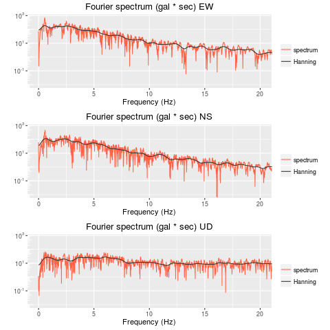
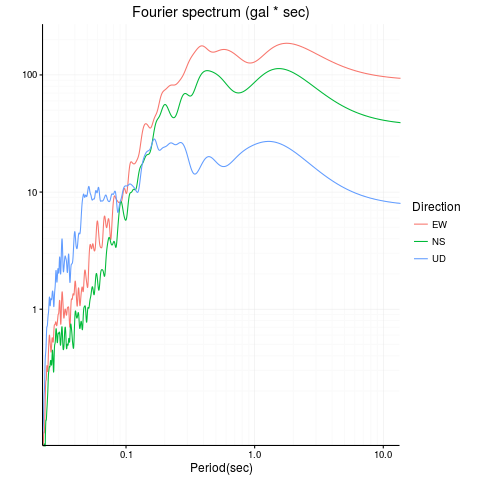
lim=max(max(resEW$fs1),max(resNS$fs1),max(resUD$fs1)) x1<-reshape2::melt(resEW,id.vars="frq") p1<-ggplot(data=x1,aes(frq,value,colour=variable)) + geom_line() p1<-p1 + scale_colour_manual(name="",labels = c(fs1= "spectrum",fs2 = "Hanning"),values = c(fs1= "tomato",fs2 = "gray20") ) p1<-p1 + scale_y_log10(labels=trans_format("log10", math_format(10^.x))) p1<-p1 + coord_cartesian(xlim=c(0,20), ylim=c(1e-2,lim)) + annotation_logticks(sides="l",colour="white") p1<-p1 + labs(x="Frequency (Hz)",y="",title="Fourier spectrum (gal * sec) EW") x1<-reshape2::melt(resNS,id.vars="frq") p2<-ggplot(data=x1,aes(frq,value,colour=variable)) + geom_line() p2<-p2 + scale_colour_manual(name="",labels = c(fs1= "spectrum",fs2 = "Hanning"),values = c(fs1= "tomato",fs2 = "gray20") ) p2<-p2 + scale_y_log10(labels=trans_format("log10", math_format(10^.x))) p2<-p2 + coord_cartesian(xlim=c(0,20), ylim=c(1e-2,lim)) + annotation_logticks(sides="l",colour="white") p2<-p2 + labs(x="Frequency (Hz)",y="",title="Fourier spectrum (gal * sec) NS") x1<-reshape2::melt(resUD,id.vars="frq") p3<-ggplot(data=x1,aes(frq,value,colour=variable)) + geom_line() p3<-p3 + scale_colour_manual(name="",labels = c(fs1= "spectrum",fs2 = "Hanning"),values = c(fs1= "tomato",fs2 = "gray20") ) p3<-p3 + scale_y_log10(labels=trans_format("log10", math_format(10^.x))) p3<-p3 + coord_cartesian(xlim=c(0,20), ylim=c(1e-2,lim)) + annotation_logticks(sides="l",colour="white") p3<-p3 + labs(x="Frequency (Hz)",y="",title="Fourier spectrum (gal * sec) UD") grid.arrange(p1,p2,p3,ncol=1)
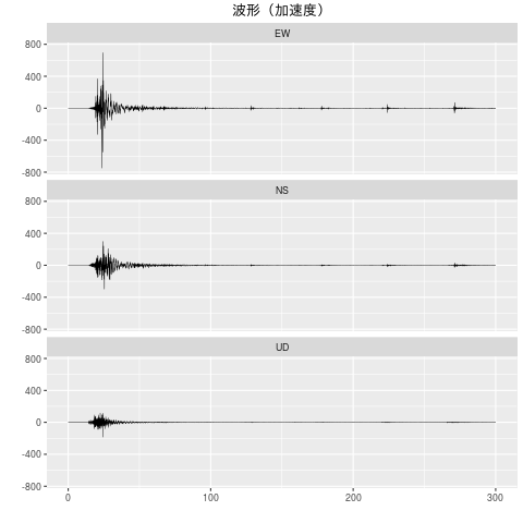
|