名目GDP推移

ggplot2 , ggfortify , grid , zoo , xts , XML パッケージ

(参考)
平成26年度国民経済計算確報(フロー編)ポイント(平成27年12月25日)(PDF)
International population pyramids with ggplot2
List of FIPS country codes

(データ)
四半期別GDP速報(2015年10-12月期 2次速報値)名目原系列(CSV形式)
日本銀行:主要時系列統計データ表(月次)
Census.gov : International Programs Data

データの加工

名目GDP &ドル・円データ
1
2
3
4
5
6
7
8
9
10
11
#名目GDP
x<-scan("clipboard")
meimokuGDP <- ts(x, start = c(1994, 1), frequency = 4)
#ドル・円 東京市場 
x<-scan("clipboard")
dy1994_2015 <- ts(x, start = c(1994, 1), frequency = 12)
library(xts)
dy.xts <- as.xts(dy1994_2015)
#ドル・円データは xts::apply.quarterly( ,mean) 関数を使って、3ヶ月(各四半期)の平均値を求め、
#四半期データを作成する(GDPデータに合わせる)
dy1994_2015_4<-ts(coredata(apply.quarterly(dy.xts,mean)),start = c(1994, 1), frequency = 4)
日本の人口
1
2
3
4
5
6
7
8
9
10
11
12
13
14
15
16
17
18
library(XML)
#日本の「FIPS country codes」は"JA"
country<-"JA"
#空のデータフレーム作成。colの数は5。
population<-read.table(text = "",col.names = c("Year","Age","BothSexes","Male","Female"))
y<-seq(1994,2015,1)
for ( i in 1:length(y)){
url<-paste0("http://www.census.gov/population/international/data/idb/region.php?N=%20Results%20&T=10&A=separate&RT=0&Y=",y[i],"&R=-1&C=",country)
df <- data.frame(readHTMLTable(url))
keep <- c(1,2,3,4,5)
df <- df[,keep]
names(df)<-c("Year","Age","BothSexes","Male","Female")
#コンマを取り除く
cols <- c(3,4,5)
df[,cols] <- apply(df[,cols], 2, function(x) as.numeric(as.character(gsub(",", "", x))))
population<-rbind(population,df)
}
popJA1994_2015<-population

グラフ作成

名目GDP
1
2
3
4
5
6
7
8
9
10
11
12
13
14
15
16
17
18
19
load(url("http://statrstart.github.io/data/dy1994_2015_4.RData"))
load(url("http://statrstart.github.io/data/meimokuGDP.RData"))
library(ggplot2)
library(ggfortify)
library(grid)
#名目GDP
p1<-autoplot(meimokuGDP)+ggtitle("名目GDP(単位:10億円)")+theme(text=element_text(size=9,family="TakaoExMincho"))
p2<-autoplot(dy1994_2015_4,size=2,colour="green")+ggtitle("ドル・円 : 東京市場 スポット") +theme(text=element_text(size=12,family="Dejima"))
#autoplotを使用しない。point+line
p3<-ggplot(data=fortify(meimokuGDP/dy1994_2015_4),aes(x=Index, y=Data))+ geom_line() +geom_point()+
theme(text=element_text(size=12,family="AoyagiKouzanFontT")) +
labs(x="",y="",title="名目GDP(ドル換算 単位:10億ドル)")
#png("gdp01.png")
grid.newpage() #空の画面を作る
pushViewport(viewport(layout=grid.layout(3,1))) #画面を区切る
print(p1,vp=viewport(layout.pos.row=1)) #1行目 , layout.pos.col=1
print(p2,vp=viewport(layout.pos.row=2)) #2行目
print(p3,vp=viewport(layout.pos.row=3)) #3行目 , layout.pos.col=1:2
#dev.off()

1
2
3
4
5
6
7
8
9
10
11
12
13
14
15
16
17
18
19
20
21
22
23
24
25
26
27
28
29
library(zoo)
z <- as.zoo(meimokuGDP)
p1<-autoplot(z) +ggtitle("名目GDP(単位:10億円)") +
theme(text=element_text(size=12,family="Sawarabi Mincho")) +
annotate("rect", fill = "red", alpha = 0.2,
xmin = 2013, xmax = 2015 + 3/4,
ymin = -Inf, ymax = Inf)
z <- as.zoo(dy1994_2015_4)
p2<-autoplot(z,colour="blue") +ggtitle("ドル・円 : 東京市場 スポット") +
theme(text=element_text(size=12,family="Sawarabi Mincho")) +
annotate("rect", fill = "red", alpha = 0.2,
xmin = 2013, xmax = 2015 + 3/4,
ymin = -Inf, ymax = Inf)
#autoplotを使用しない。point+line
z <- as.zoo(meimokuGDP/dy1994_2015_4)
p3<-ggplot(aes(x = Index, y = Value), data = fortify(z, melt = TRUE)) +
geom_line() +geom_point()+
theme(text=element_text(size=12,family="Sawarabi Mincho")) +
annotate("rect", fill = "red", alpha = 0.2,
xmin = 2013, xmax = 2015 + 3/4,
ymin = -Inf, ymax = Inf) +
labs(x="",y="",title="名目GDP(ドル換算 単位:10億ドル)")
#png("gdp02.png")
grid.newpage() #空の画面を作る
pushViewport(viewport(layout=grid.layout(3,1))) #画面を区切る
print(p1,vp=viewport(layout.pos.row=1)) #1行目
print(p2,vp=viewport(layout.pos.row=2)) #2行目
print(p3,vp=viewport(layout.pos.row=3)) #3行目
#dev.off()

暦年
1
2
3
4
5
6
7
8
9
10
11
12
13
14
15
16
17
18
19
20
21
22
23
24
25
26
library(xts)
#xts::apply.yearly( ,sum) 関数を使って、四半期の合計を求め、暦年データを作成する
data1 <- apply.yearly(as.xts(meimokuGDP),sum)
data2 <- apply.yearly(as.xts(meimokuGDP/dy1994_2015_4),sum)
#p1<-ggplot(data =fortify(data1,melt=TRUE),aes(x = Index, y = Value)) +
p1<-ggplot(data =fortify(data1,melt=TRUE),aes(x =seq(1994,2015), y = Value)) +
geom_line() +geom_point()+
theme(text=element_text(size=12,family="TakaoPGothic")) +
annotate("rect", fill = "red", alpha = 0.2,
xmin = 2013-1/2, xmax = 2015 + 1/2,
ymin = -Inf, ymax = Inf) +
labs(x="",y="",title="名目GDP(単位:10億円)")
#p2<-ggplot(data =fortify(data2.xts,melt=TRUE),aes(x = Index, y = Value)) +
p2<-ggplot(data =fortify(data2,melt=TRUE),aes(x = seq(1994,2015), y = Value)) +
geom_line() +geom_point()+
theme(text=element_text(size=12,family="Droid Sans Japanese")) +
annotate("rect", fill = "red", alpha = 0.2,
xmin = 2013-1/2, xmax = 2015 + 1/2,
ymin = -Inf, ymax = Inf) +
labs(x="",y="",title="名目GDP(ドル換算 単位:10億ドル)")
#png("gdp03.png")
grid.newpage() #空の画面を作る
pushViewport(viewport(layout=grid.layout(2,1))) #画面を区切る
print(p1,vp=viewport(layout.pos.row=1)) #1行目
print(p2,vp=viewport(layout.pos.row=2)) #2行目
#dev.off()

国民一人あたり名目GDP
1
2
3
4
5
6
7
8
9
10
11
12
13
14
15
16
17
18
19
20
21
22
23
24
25
26
27
28
29
load(url("http://statrstart.github.io/data/popJA1994_2015.RData"))
df <- popJA1994_2015[popJA1994_2015$Age=="Total",]
#人口は年次データ rep(df$BothSexes,each=4) として四半期データに合わせる。
#国民一人あたり名目GDP(円)
yen<-(meimokuGDP)*1e+9/ts(rep(df$BothSexes,each=4),start=1994,freq=4)
#国民一人あたり名目GDP(ドル換算)
dol<-(meimokuGDP/dy1994_2015_4)*1e+9/ts(rep(df$BothSexes,each=4),start=1994,freq=4)
#国民一人あたり名目GDP(円)
z <- data.frame(as.matrix(time(yen)),as.matrix(yen))
names(z)<-c("date","gdp")
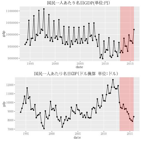
p1<-ggplot(data=z,aes(x=date, y=gdp))+ geom_line() +geom_point()+
theme(text=element_text(size=12,family="IPAexMincho")) +
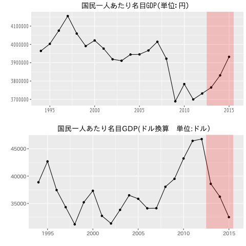
ggtitle("国民一人あたり名目GDP(単位:円)") +
annotate("rect", fill = "red", alpha = 0.2,
xmin=2013,xmax=2015 + 3/4,ymin=-Inf,ymax=Inf )
#国民一人あたり名目GDP(ドル換算)
z <- data.frame(as.matrix(time(dol)),as.matrix(dol))
names(z)<-c("date","gdp")
p2<-ggplot(data=z,aes(x=date, y=gdp))+ geom_line() +geom_point()+
theme(text=element_text(size=12,family="Ume Mincho")) +
ggtitle("国民一人あたり名目GDP(ドル換算 単位:ドル)") +
annotate("rect", fill = "red", alpha = 0.2,
xmin=2013,xmax=2015 + 3/4,ymin=-Inf,ymax=Inf )
#png("gdp04.png")
grid.newpage() #空の画面を作る
pushViewport(viewport(layout=grid.layout(2,1))) #画面を区切る
print(p1,vp=viewport(layout.pos.row=1)) #1行目
print(p2,vp=viewport(layout.pos.row=2)) #2行目
#dev.off()

暦年
1
2
3
4
5
6
7
8
9
10
11
12
13
14
15
16
17
18
19
20
21
22
23
24
25
26
library(xts)
#xts::apply.yearly( ,sum) 関数を使って、四半期の合計を求め、暦年データを作成する
data1 <- apply.yearly(as.xts(yen),sum)
data2 <- apply.yearly(as.xts(dol),sum)
#p1<-ggplot(data =fortify(data1,melt=TRUE),aes(x = Index, y = Value)) +
p1<-ggplot(data =fortify(data1,melt=TRUE),aes(x =seq(1994,2015), y = Value)) +
geom_line() +geom_point()+
theme(text=element_text(size=12,family="Ume Gothic S4")) +
annotate("rect", fill = "red", alpha = 0.2,
xmin = 2013-1/2, xmax = 2015 + 1/2,
ymin = -Inf, ymax = Inf) +
labs(x="",y="",title="国民一人あたり名目GDP(単位:円)")
#p2<-ggplot(data =fortify(data2,melt=TRUE),aes(x = Index, y = Value)) +
p2<-ggplot(data =fortify(data2,melt=TRUE),aes(x = seq(1994,2015), y = Value)) +
geom_line() +geom_point()+
theme(text=element_text(size=12,family="IPAexGothic")) +
annotate("rect", fill = "red", alpha = 0.2,
xmin = 2013-1/2, xmax = 2015 + 1/2,
ymin = -Inf, ymax = Inf) +
labs(x="",y="",title="国民一人あたり名目GDP(ドル換算 単位:ドル)")
#png("gdp05.png")
grid.newpage() #空の画面を作る
pushViewport(viewport(layout=grid.layout(2,1))) #画面を区切る
print(p1,vp=viewport(layout.pos.row=1)) #1行目
print(p2,vp=viewport(layout.pos.row=2)) #2行目
#dev.off()