riverplot パッケージ
(参考)環境省『平成25年版環境・循環型社会・生物多様性白書』
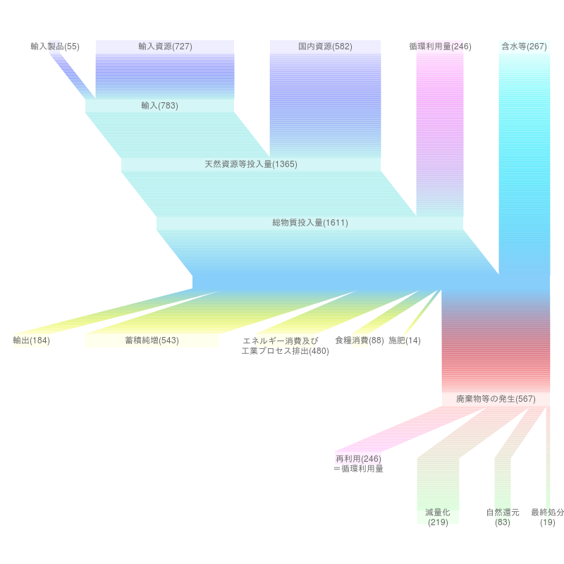
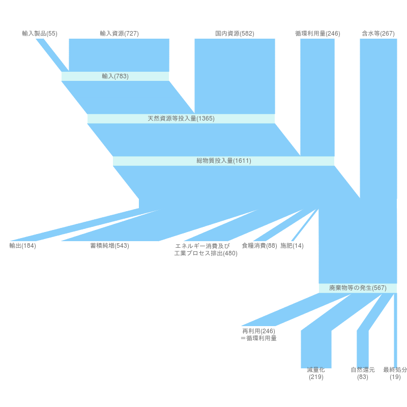
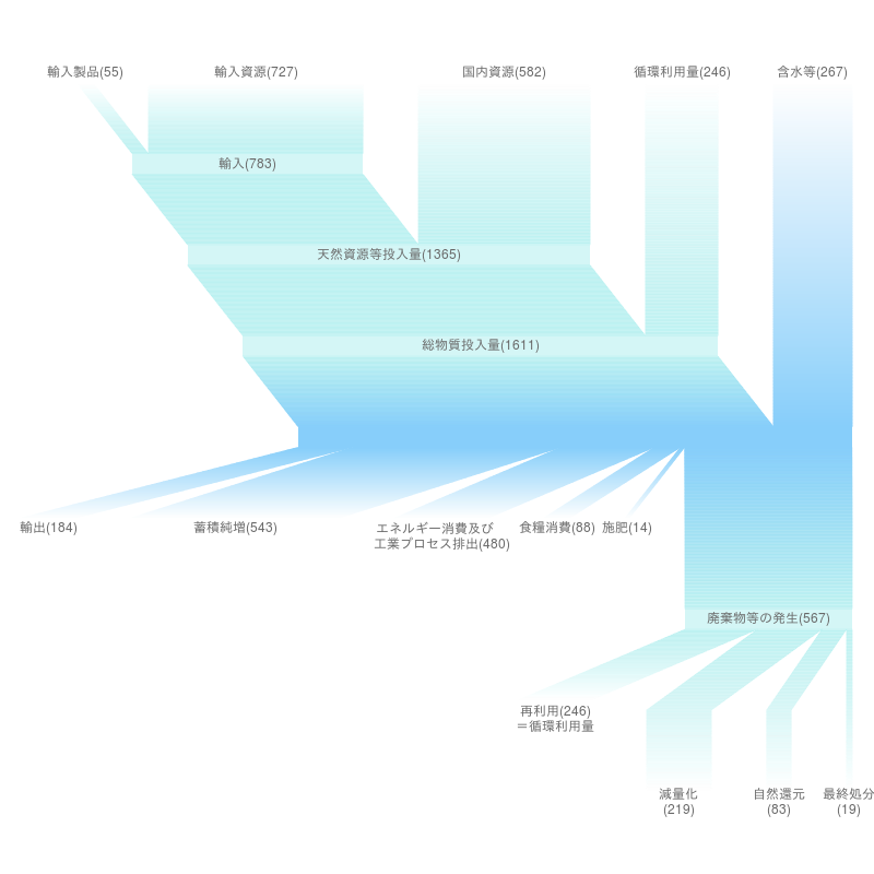
我が国の物質フロー平成22年度
|
|
N1 N2 Value
1 輸入製品 輸入 55
2 輸入資源 輸入 727
3 輸入 天然資源等投入量 783
4 国内資源 天然資源等投入量 582
5 天然資源等投入量 総物質投入量 1365
6 循環利用量 総物質投入量 246
7 総物質投入量 投入総量 1611
8 含水等 投入総量 267
9 投入総量 輸出 184
10 投入総量 蓄積純増 706
11 投入総量 エネルギー消費及び工業プロセス排出 317
12 投入総量 食糧消費 88
13 投入総量 施肥 14
14 投入総量 廃棄物等の発生 567
15 廃棄物等の発生 再利用 246
16 廃棄物等の発生 減量化 219
17 廃棄物等の発生 自然還元 83
18 廃棄物等の発生 最終処分 19
|
|
ID x
1 輸入製品 1
2 輸入資源 1
3 輸入 2
4 国内資源 1
5 天然資源等投入量 3
6 循環利用量 1
7 総物質投入量 4
8 含水等 1
9 投入総量 5
10 廃棄物等の発生 7
11 輸出 6
12 蓄積純増 6
13 エネルギー消費及び工業プロセス排出 6
14 食糧消費 6
15 施肥 6
16 再利用 8
17 減量化 9
18 自然還元 9
19 最終処分 9
|
|
時計回りに90度回転(以下のグラフも同じ)
ラベルを指定
|
|
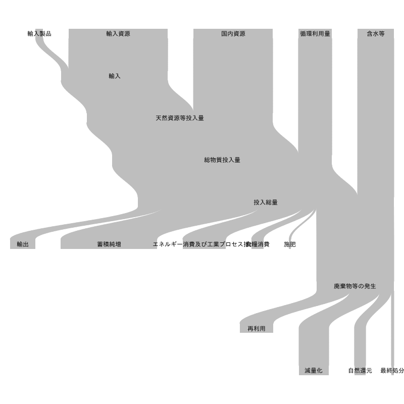
stylesも指定する(1)
|
|
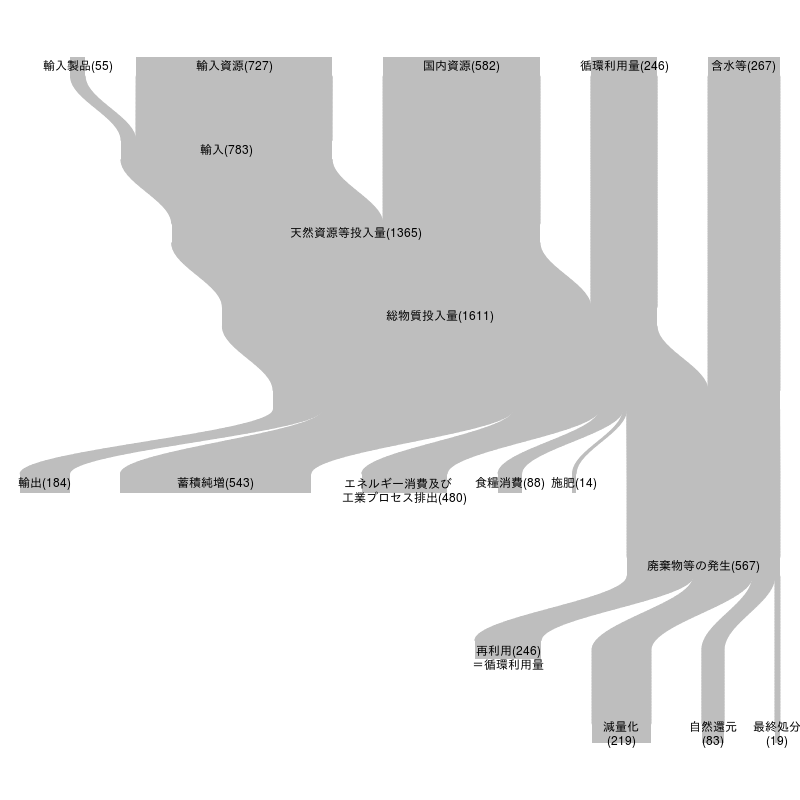
stylesも指定する(2)
|
|
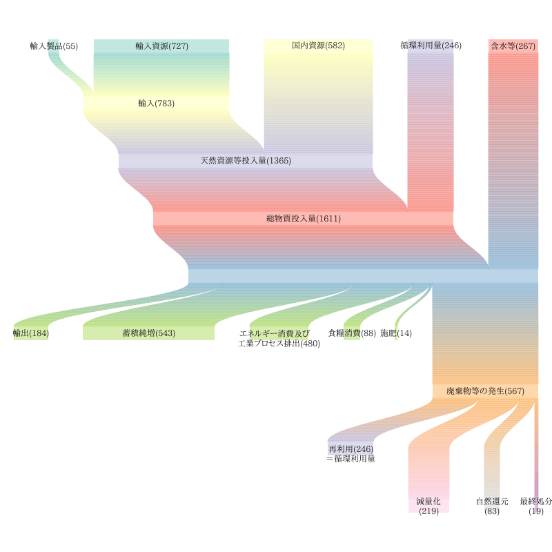
stylesも指定する(3)
|
|
stylesも指定する(4)
|
|