Jul 5 2015

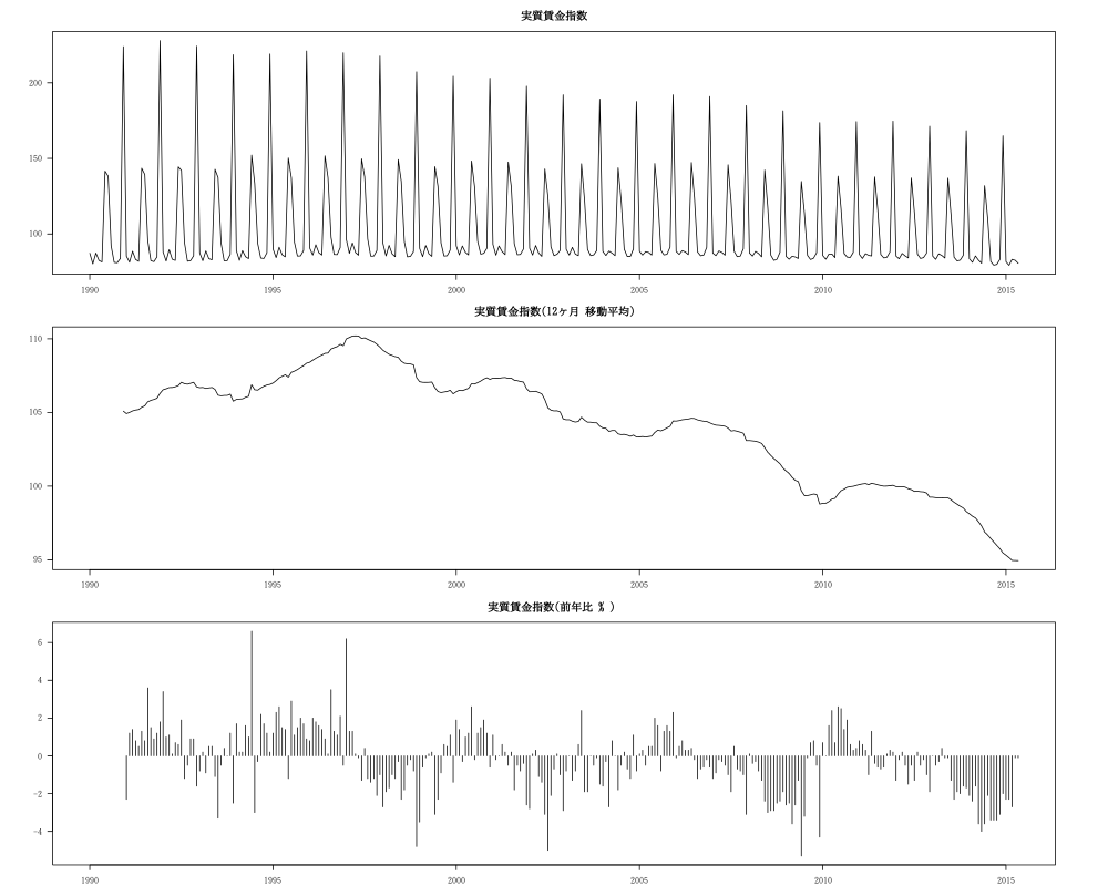
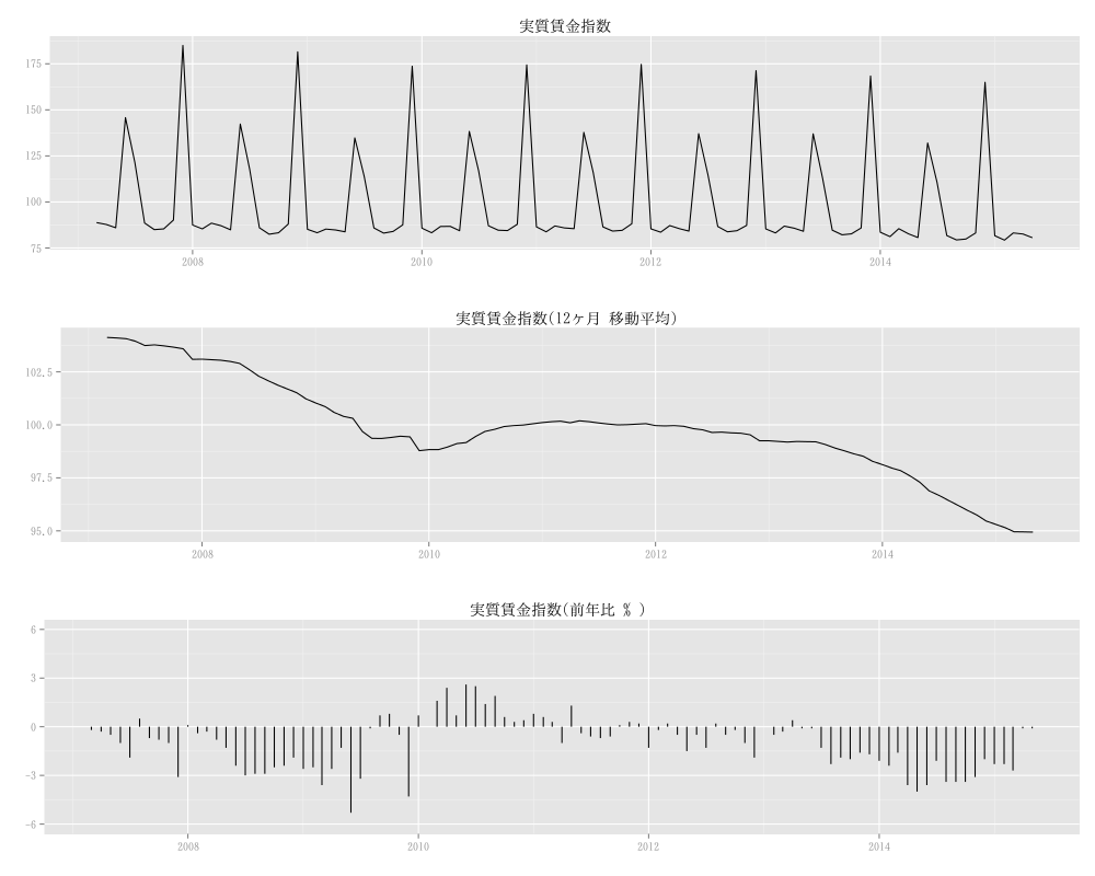
毎月勤労統計調査2

ts class

OSはzorin os

毎月勤労統計調査　全国調査長期時系列表月次 2月
実質賃金　指数及び増減率－現金給与総額（５人以上）（調査産業計）(公表日 2015年4月17日)に
毎月勤労統計調査　全国調査月次-2015年5月(公表日 2015年6月30日)の5月速報値(時系列第6表　実質賃金指数)を追加。

エクセルファイルの取り込む箇所をコピーして「scan(“clipboard”)」で取り込むのが結局は一番楽。

2015年5月分は速報値

library(TTR)
#Industries_covered<-scan("clipboard")
Industries_covered<-c(87.3,80.3,87.4,82.5,81.5,141.6,138.3,92.2,81.2,81.0,83.8,224.0,85.3,81.3,88.6,83.2,81.9,143.5,139.4,95.5,82.4,81.7,
84.8,228.0,88.2,82.1,89.6,83.3,82.5,144.4,142.1,94.4,82.0,82.4,85.6,224.3,87.5,82.3,88.8,83.7,82.9,142.8,137.4,93.9,
82.3,82.4,86.6,218.6,89.0,82.5,89.0,85.0,83.7,152.2,133.3,93.6,84.1,83.8,87.6,219.1,90.1,84.4,91.3,86.3,84.9,150.3,
137.2,94.6,85.4,85.5,89.1,221.1,90.8,86.1,92.9,87.7,86.1,151.7,137.4,97.9,86.5,86.4,91.0,219.9,96.4,87.2,94.1,87.8,
86.0,149.7,137.9,96.7,85.3,85.4,89.1,217.7,93.8,85.5,92.5,86.9,85.0,149.2,134.7,95.0,84.9,85.2,88.4,207.3,90.5,85.0,
92.4,87.0,85.2,144.6,131.6,94.1,85.4,85.6,89.4,204.4,92.2,86.2,92.1,87.9,86.2,148.3,131.4,95.2,86.7,87.2,90.5,203.1,
93.2,86.0,92.1,88.4,86.4,147.6,131.6,93.5,86.3,86.5,90.1,197.8,90.6,86.1,92.4,87.4,85.2,143.0,125.0,91.5,85.7,86.6,
89.2,192.1,89.9,86.1,91.2,86.7,85.7,146.5,122.6,89.8,85.7,86.2,89.1,189.3,88.5,85.8,88.7,87.4,85.7,143.8,122.0,90.0,
85.1,85.2,90.1,187.7,88.6,86.1,88.3,87.8,86.1,146.7,124.0,89.3,86.2,86.6,91.3,192.1,88.5,86.5,89.0,88.1,86.4,147.3,
123.8,88.2,85.6,86.1,91.1,191.0,87.4,85.7,88.8,87.8,86.0,145.8,121.4,88.6,85.0,85.4,90.2,185.0,87.5,85.4,88.5,87.1,
84.9,142.3,117.7,86.0,82.5,83.3,88.0,181.5,85.2,83.3,85.3,84.8,83.8,134.8,113.9,85.9,83.1,84.0,87.6,173.7,85.8,83.3,
86.7,86.8,84.4,138.3,116.7,87.1,84.7,84.5,87.9,174.4,86.5,83.8,87.0,85.9,85.5,137.8,116.0,86.5,84.2,84.6,88.2,174.7,
85.4,83.6,87.2,85.5,84.2,137.1,114.5,86.7,83.8,84.4,87.3,171.3,85.4,83.2,86.9,85.8,84.1,137.0,113.0,84.7,82.2,82.7,
85.9,168.4,83.6,81.2,85.5,82.7,80.7,132.0,110.6,81.8,79.4,79.9,83.2,165.0,81.7,79.3,83.2,82.6,80.6)
Industries_covered.ts<-ts(Industries_covered,start=1990,freq=12)
#YeaOnYear_growth_rates<-scan("clipboard")
YeaOnYear_growth_rates<-c(-2.3,1.2,1.4,0.8,0.5,1.3,0.8,3.6,1.5,0.9,1.2,1.8,3.4,1.0,1.1,0.1,0.7,0.6,1.9,-1.2,-0.5,0.9,0.9,-1.6,-0.8,0.2,-0.9,
0.5,0.5,-1.1,-3.3,-0.5,0.4,0.0,1.2,-2.5,1.7,0.2,0.2,1.6,1.0,6.6,-3.0,-0.3,2.2,1.7,1.2,0.2,1.2,2.3,2.6,1.5,1.4,-1.2,
2.9,1.1,1.5,2.0,1.7,0.9,0.8,2.0,1.8,1.6,1.4,0.9,0.1,3.5,1.3,1.1,2.1,-0.5,6.2,1.3,1.3,0.1,-0.1,-1.3,0.4,-1.2,-1.4,
-1.2,-2.1,-1.0,-2.7,-1.9,-1.7,-1.0,-1.2,-0.3,-2.3,-1.8,-0.5,-0.2,-0.8,-4.8,-3.5,-0.6,-0.1,0.1,0.2,-3.1,-2.3,-0.9,0.6,0.5,1.1,-1.4,
1.9,1.4,-0.3,1.0,1.2,2.6,-0.2,1.2,1.5,1.9,1.2,-0.6,1.1,-0.2,0.0,0.6,0.2,-0.5,0.2,-1.8,-0.5,-0.8,-0.4,-2.6,-2.8,0.1,0.3,
-1.1,-1.4,-3.1,-5.0,-2.1,-0.7,0.1,-1.0,-2.9,-0.8,0.0,-1.3,-0.8,0.6,2.4,-1.9,-1.9,0.0,-0.5,-0.1,-1.5,-1.6,-0.3,-2.7,0.8,0.0,-1.8,
-0.5,0.2,-0.7,-1.2,1.1,-0.8,0.1,0.3,-0.5,0.5,0.5,2.0,1.6,-0.8,1.3,1.6,1.3,2.3,-0.1,0.5,0.8,0.3,0.3,0.4,-0.2,-1.2,-0.7,
-0.6,-0.2,-0.6,-1.2,-0.9,-0.2,-0.3,-0.5,-1.0,-1.9,0.5,-0.7,-0.8,-1.0,-3.1,0.1,-0.4,-0.3,-0.8,-1.3,-2.4,-3.0,-2.9,-2.9,-2.5,-2.4,-1.9,
-2.6,-2.5,-3.6,-2.6,-1.3,-5.3,-3.2,-0.1,0.7,0.8,-0.5,-4.3,0.7,0.0,1.6,2.4,0.7,2.6,2.5,1.4,1.9,0.6,0.3,0.4,0.8,0.6,0.3,
-1.0,1.3,-0.4,-0.6,-0.7,-0.6,0.1,0.3,0.2,-1.3,-0.2,0.2,-0.5,-1.5,-0.5,-1.3,0.2,-0.5,-0.2,-1.0,-1.9,0.0,-0.5,-0.3,0.4,-0.1,-0.1,
-1.3,-2.3,-1.9,-2.0,-1.6,-1.7,-2.1,-2.4,-1.6,-3.6,-4.0,-3.6,-2.1,-3.4,-3.4,-3.4,-3.1,-2.0,-2.3,-2.3,-2.7,-0.1,-0.1)
#縦軸をそろえるため1990年分NAを12個追加
YeaOnYear_growth_rates<-c(rep(NA,12),YeaOnYear_growth_rates)
YeaOnYear_growth_rates.ts<-ts(YeaOnYear_growth_rates,start=1990,freq=12)
#plot(plot.ts)
#png("Ic01.png",width=1000,height=800)
#par(family="TakaoMincho",mfrow=c(3,1),mar = c(2, 5, 3, 5))
par(mfrow=c(3,1),mar = c(2, 5, 3, 5))
plot(Industries_covered.ts,las=1,main="実質賃金指数",ylab="")
plot(SMA(Industries_covered.ts,12),las=1,main="実質賃金指数(12ヶ月 移動平均)",ylab="")
#lend=1でlineの端をその値で平坦に！
plot(YeaOnYear_growth_rates.ts,type="h",lend=1,las=1,main="実質賃金指数(前年比 % ）",ylab="")
par(mfrow=c(1,1))
#dev.off()

関数windowを用いて、時系列の一部分(2007/3～2015/5)を切り出す。

ggplot2を使う。フォントの変更方法が通常のプロットとは異なる。

(参考)
ggplot2 はじめの一歩

library(ggplot2)
library(gridExtra)
old = theme_set(theme_gray(base_family="TakaoMincho"))
#png("Ic02.png",width=1000,height=800)
df <- data.frame(date=as.Date(time(window(Industries_covered.ts,c(2007,3),c(2015,5)))), 
y=as.matrix(window(Industries_covered.ts,c(2007,3),c(2015,5))))
p1<-ggplot(df,aes(x=date,y=y))+geom_line()+labs(x="",y="",title="実質賃金指数")
df <- df <- data.frame(date=as.Date(time(window(SMA(Industries_covered.ts,12),c(2007,3),c(2015,5)))), 
y=as.matrix(window(SMA(Industries_covered.ts,12),c(2007,3),c(2015,5))))
p2<-ggplot(df,aes(x=date,y=y))+geom_line()+labs(x="",y="",title="実質賃金指数(12ヶ月 移動平均）")
df <- data.frame(date=as.Date(time(window(YeaOnYear_growth_rates.ts,c(2007,3),c(2015,5)))), 
y=as.matrix(window(YeaOnYear_growth_rates.ts,c(2007,3),c(2015,5))))
p3<-ggplot(df,aes(x=date,xend=date,y=0,yend=y))+geom_segment()+labs(x="",y="",title="実質賃金指数(前年比 % ）")+ylim(-6,6)
grid.arrange(p1,p2,p3,ncol=1,nrow=3)
#dev.off()

民主党政権3年3ヶ月(2009年9月16日から2012年12月26日)
消費税 8％ (2014年4月1日)

東大指数（日次物価指数、日次売上高指数）

#日次物価指数
prices <- read.csv("http://www.cmdlab.co.jp/price_u-tokyo/download/HistoricalDailyData.csv", header=TRUE,na.strings="NA",stringsAsFactors = F)
head(prices)
#日次売上高指数
sales <- read.csv("http://www.cmdlab.co.jp/price_u-tokyo/download/SalesDailyData.csv", header=TRUE,na.strings="NA",stringsAsFactors = F)
head(sales)
library(TTR)
#
#png("Ic03.png",width=1000,height=800)
#par(family="TakaoMincho",mfrow=c(3,1),mar = c(2, 5, 3, 5))
#par(mfrow=c(3,1),mar = c(2, 5, 3, 5))
prices.xts <- as.xts(zoo(prices[,-1]), as.POSIXct(prices$date))
plot.zoo(prices.xts["2007-03-01::",2],main="東大物価指数(2007-03-01～)",xlab="",ylab="",las=1,ylim=c(-0.04,0.04))
abline(h=0,col="red",lty=3)
#
#sales$X7dayaverage<-as.numeric(as.vector(sales$X7dayaverage))
sales$X7dayaverage<-as.numeric(sales$X7dayaverage)
sales.xts <- as.xts(zoo(sales[,-1]), as.POSIXct(sales$date))
plot.zoo(SMA(sales.xts["2007-03-01::",2],28),main="東大売上高指数(2007-03-01～)",xlab="",ylab="",las=1,ylim=c(-0.08,0.08))
abline(h=0,col="red",lty=3)
#
Industries_covered<-c(87.3,80.3,87.4,82.5,81.5,141.6,138.3,92.2,81.2,81.0,83.8,224.0,85.3,81.3,88.6,83.2,81.9,143.5,139.4,95.5,82.4,81.7,
84.8,228.0,88.2,82.1,89.6,83.3,82.5,144.4,142.1,94.4,82.0,82.4,85.6,224.3,87.5,82.3,88.8,83.7,82.9,142.8,137.4,93.9,
82.3,82.4,86.6,218.6,89.0,82.5,89.0,85.0,83.7,152.2,133.3,93.6,84.1,83.8,87.6,219.1,90.1,84.4,91.3,86.3,84.9,150.3,
137.2,94.6,85.4,85.5,89.1,221.1,90.8,86.1,92.9,87.7,86.1,151.7,137.4,97.9,86.5,86.4,91.0,219.9,96.4,87.2,94.1,87.8,
86.0,149.7,137.9,96.7,85.3,85.4,89.1,217.7,93.8,85.5,92.5,86.9,85.0,149.2,134.7,95.0,84.9,85.2,88.4,207.3,90.5,85.0,
92.4,87.0,85.2,144.6,131.6,94.1,85.4,85.6,89.4,204.4,92.2,86.2,92.1,87.9,86.2,148.3,131.4,95.2,86.7,87.2,90.5,203.1,
93.2,86.0,92.1,88.4,86.4,147.6,131.6,93.5,86.3,86.5,90.1,197.8,90.6,86.1,92.4,87.4,85.2,143.0,125.0,91.5,85.7,86.6,
89.2,192.1,89.9,86.1,91.2,86.7,85.7,146.5,122.6,89.8,85.7,86.2,89.1,189.3,88.5,85.8,88.7,87.4,85.7,143.8,122.0,90.0,
85.1,85.2,90.1,187.7,88.6,86.1,88.3,87.8,86.1,146.7,124.0,89.3,86.2,86.6,91.3,192.1,88.5,86.5,89.0,88.1,86.4,147.3,
123.8,88.2,85.6,86.1,91.1,191.0,87.4,85.7,88.8,87.8,86.0,145.8,121.4,88.6,85.0,85.4,90.2,185.0,87.5,85.4,88.5,87.1,
84.9,142.3,117.7,86.0,82.5,83.3,88.0,181.5,85.2,83.3,85.3,84.8,83.8,134.8,113.9,85.9,83.1,84.0,87.6,173.7,85.8,83.3,
86.7,86.8,84.4,138.3,116.7,87.1,84.7,84.5,87.9,174.4,86.5,83.8,87.0,85.9,85.5,137.8,116.0,86.5,84.2,84.6,88.2,174.7,
85.4,83.6,87.2,85.5,84.2,137.1,114.5,86.7,83.8,84.4,87.3,171.3,85.4,83.2,86.9,85.8,84.1,137.0,113.0,84.7,82.2,82.7,
85.9,168.4,83.6,81.2,85.5,82.7,80.7,132.0,110.6,81.8,79.4,79.9,83.2,165.0,81.7,79.3,83.2,82.6,80.6)
Industries_covered.ts<-ts(Industries_covered,start=1990,freq=12)
plot(window(SMA(Industries_covered.ts,12),c(2007,3),c(2015,5)),las=1,main="実質賃金指数(12ヶ月 移動平均)",xlab="",ylab="")
abline(h=100,col="red",lty=3)
par(mfrow=c(1,1))
#dev.off()