Quandl、xts、lattice、latticeExtra、gridExtra パッケージ
「21世紀の資本」のデータが公開されてるのでRを使ってグラフ化してみます。
(グラフもすでに公開されているのであまり意味はありません。)
(参考)
Piketty Codes
『21世紀の資本』日本語版サポートページ
Chapter 2: Growth: Illusions and Realities
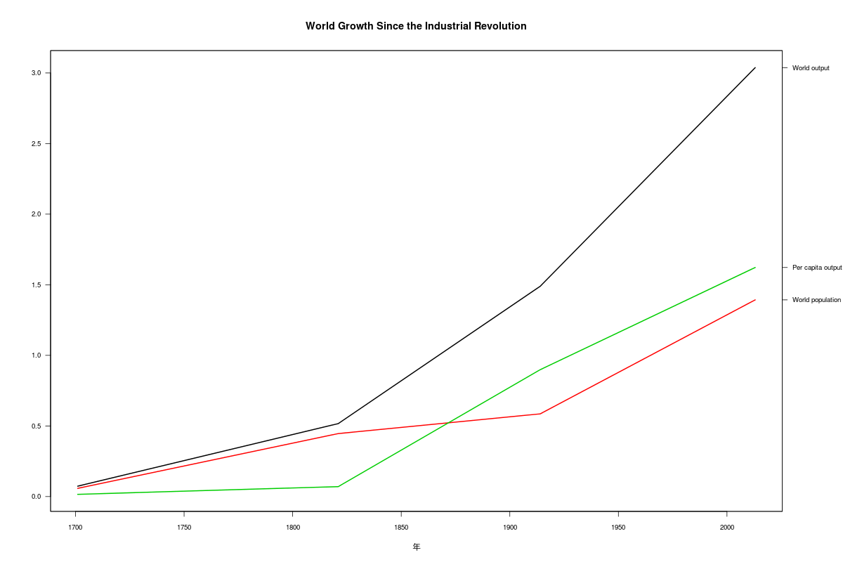
World Growth Since the Industrial Revolution
|
|
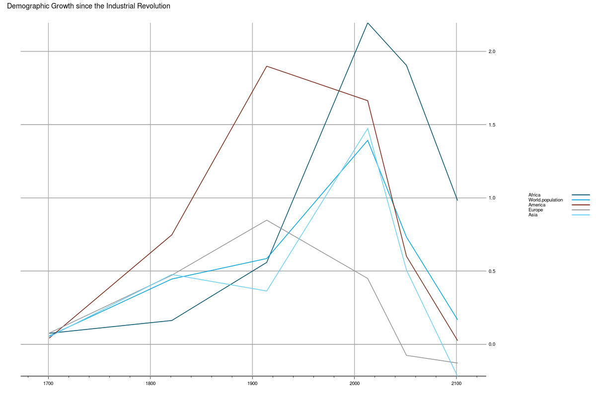
Demographic Growth since the Industrial Revolution
|
|
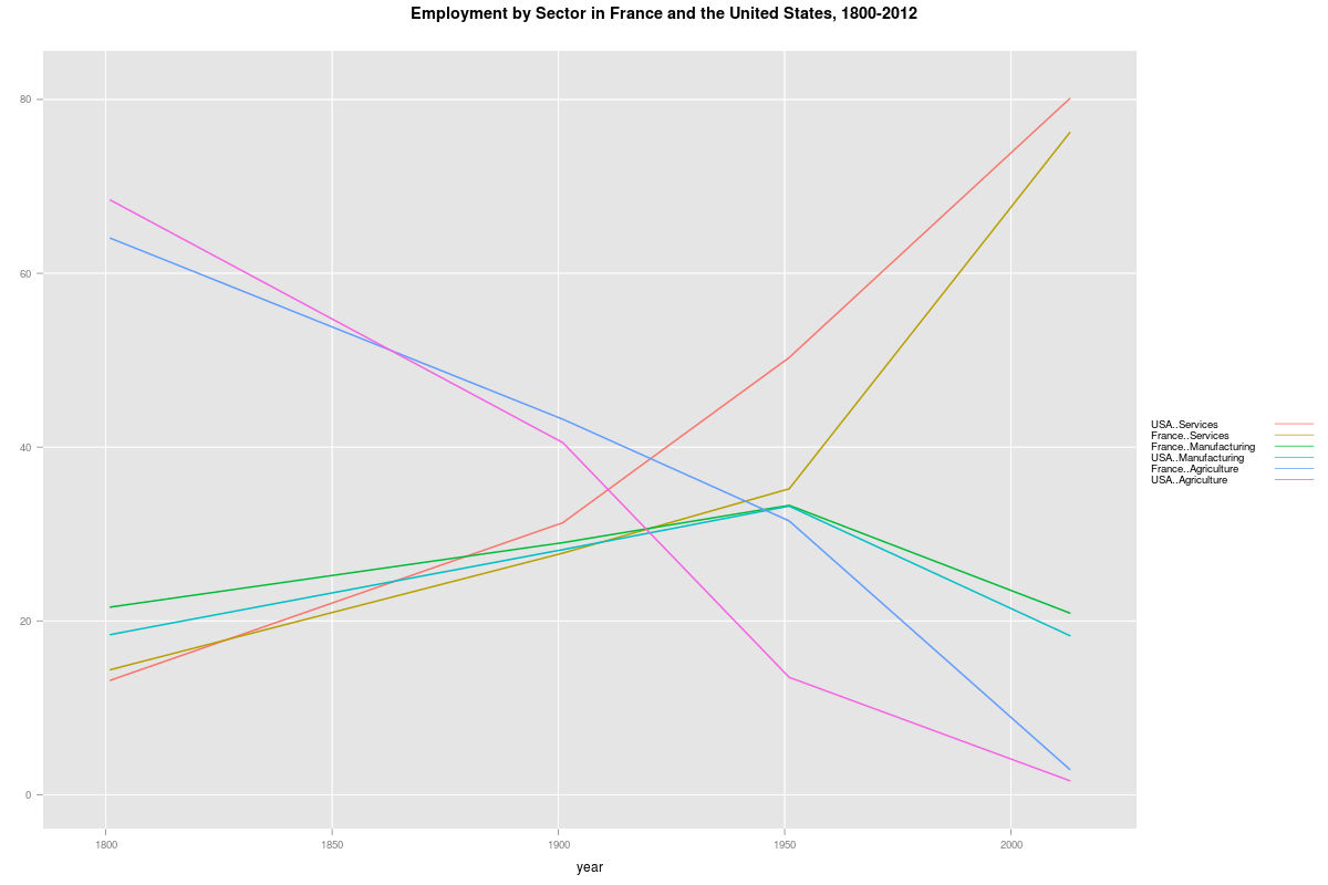
Employment by Sector in France and the United States, 1800-2012
|
|
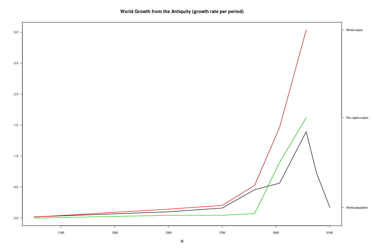
World Growth from the Antiquity (growth rate per period)
|
|
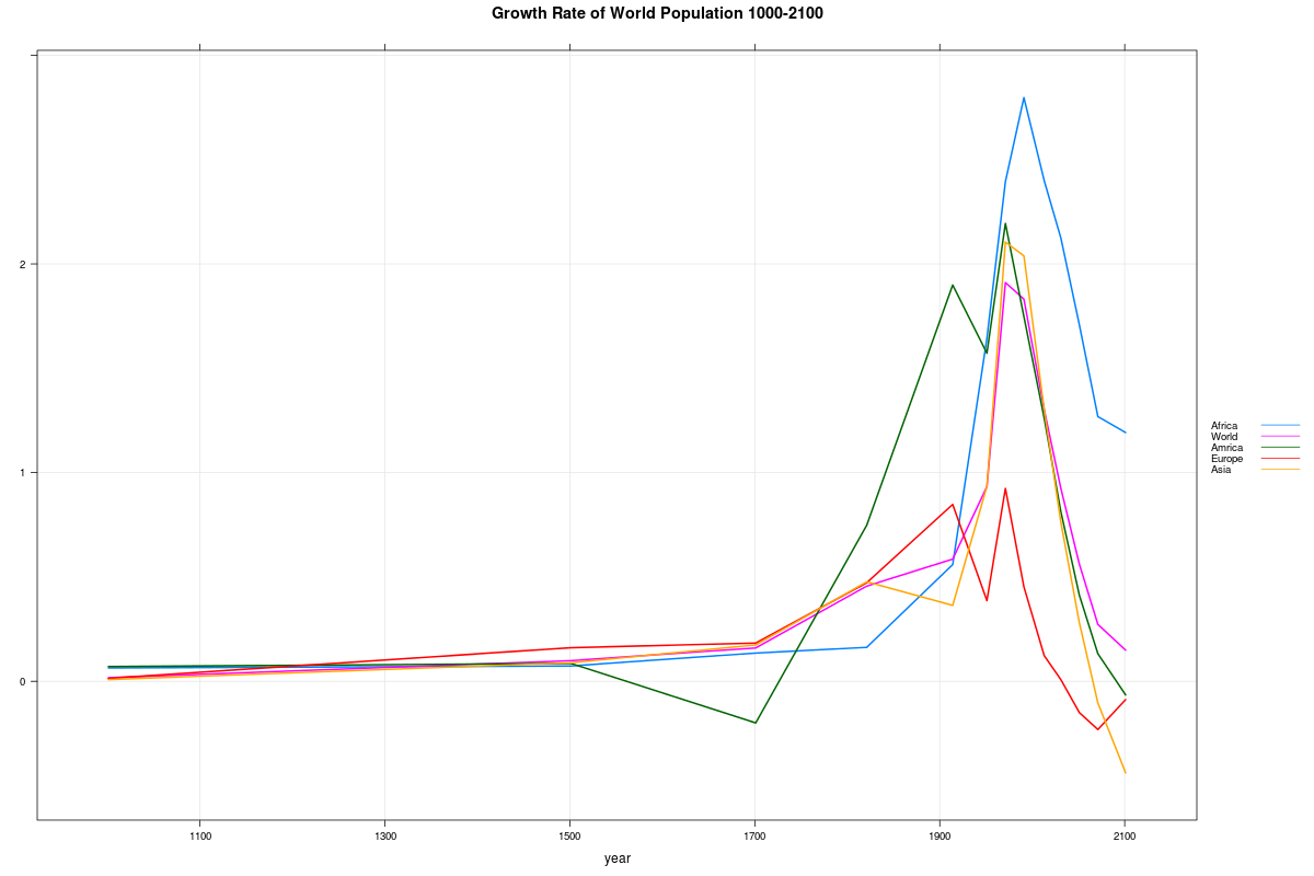
Growth Rate of World Population 1000-2100
|
|
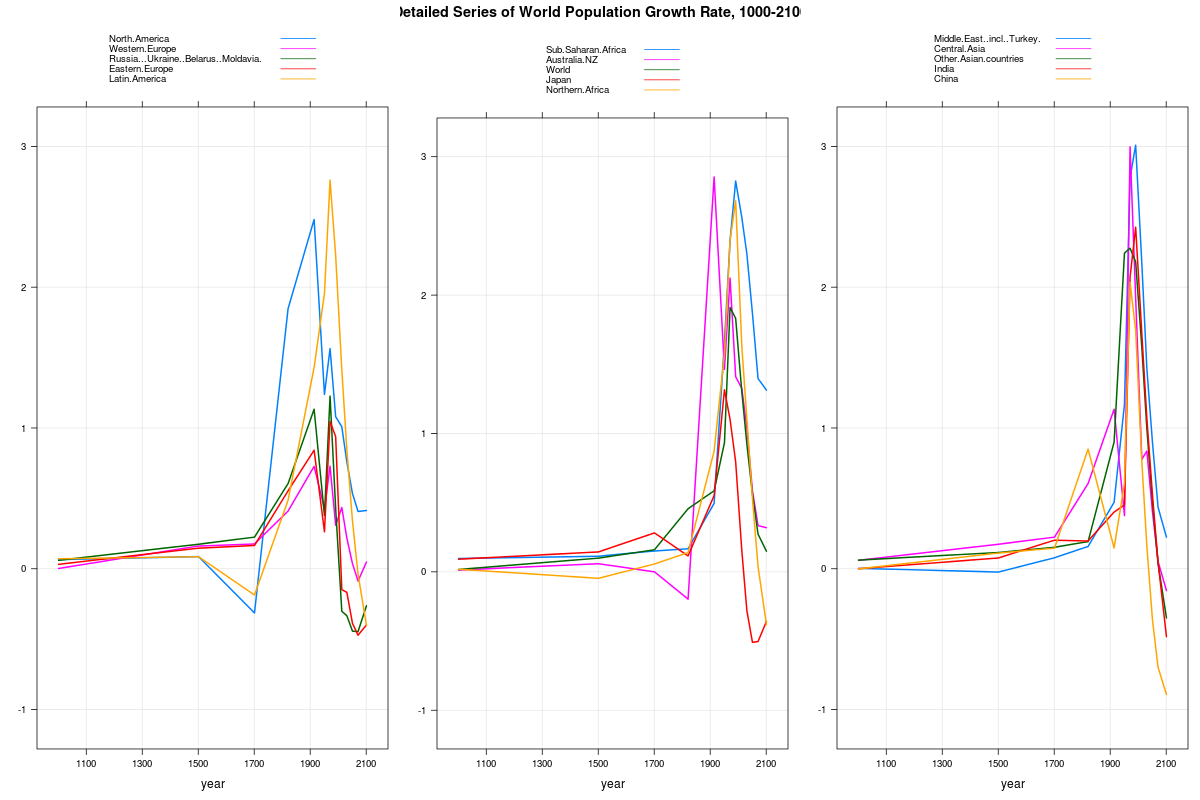
Detailed Series of World Population Growth Rate, 0-2100
|
|
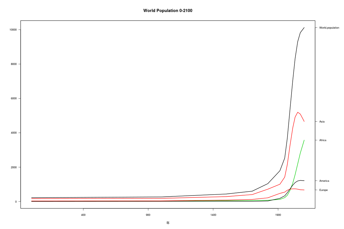
World Population 0-2100
|
|
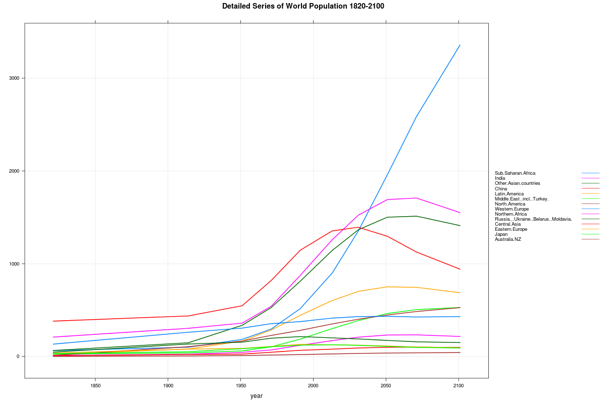
Detailed Series of World Population 0-2100
|
|
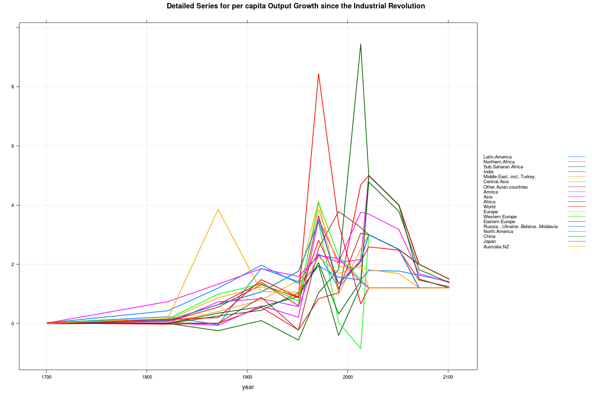
Detailed Series for per capita Output Growth since the Industrial Revolution
|
|
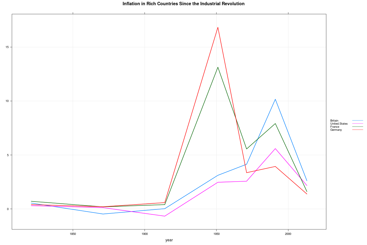
Inflation in Rich Countries Since the Industrial Revolution
|
|