家計調査2

ggplot2,reshape2 パッケージ

家計調査 家計収支編 二人以上の世帯 詳細結果表 年次
2-6 年間収入階級別（全国・全都市・都市階級） 二人以上の世帯
年間収入階級別１世帯当たり１か月間の収入（農林漁家世帯を含む）
全国:世帯数分布(抽出率調整) を抽出(2000年～2013年)

家計調査と日経500では「勤労者世帯」でしたが今回は「農林漁家世帯を含む」です

ヘッダーをつけて保存。～が文字化けするのでloadしてから、つけ直す。
データ置いときます。
＊linux用(windowsで読みこめるかは不明).間違いがあるかもしれません。

KakeiRank.dat

library(ggplot2)
library(reshape2)
load("KakeiRank.dat")
names(KakeiRank)<-c("年","２００万円未満","２００～２５０",	"２５０～３００","３００～３５０","３５０～４００","４００～４５０","４５０～５００","５００～５５０","５５０～６００","６００～６５０","６５０～７００","７００～７５０","７５０～８００","８００～９００","９００～１０００","１０００～１２５０","１２５０～１５００","１５００万円以上")
temp<-melt(KakeiRank,measure=-1)
#中央値をわかりやすく
#2013年のデータを抽出
temp1 <- subset(temp, subset=年==2013)
#並び順を示すために番号付けが必要
temp1$No<-c(1:18)
#cumsum:累計を求める
temp1$cumsum<-cumsum(temp1$value)
#
ggplot(data=temp1)+
geom_bar(stat="identity", position = "dodge",aes(x=reorder(variable,No),y=value,group=variable,fill=variable),alpha=0.9)+
geom_hline(aes(yintercept=5000), colour="gray40", linetype="dashed",alpha=0.9)+
geom_line(aes(x=No,y=cumsum),color="gray20",alpha=0.9)+
xlab("年間収入")+
ylab("世帯数（1万世帯あたり）")+
ggtitle("年間収入金額別世帯数割合と累計（1万世帯あたり）(2013年)") +
theme(legend.position = "no",axis.text.x = element_text(angle = 45, hjust = 1))
#ggsave("KRC2013.png",dpi = 100, width = 8, height = 6)

2013年

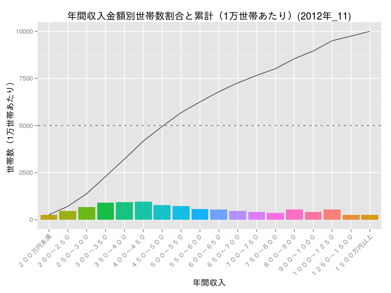
2012年

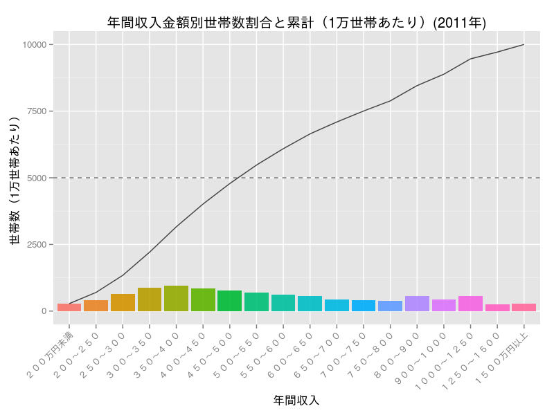
2011年

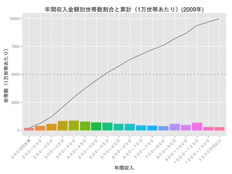
2009年 ＊9月：政権交代

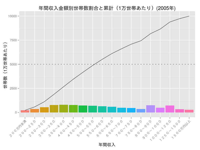
2005年

• 中央値約55０万円。第1四分位数約350～４００万円

2000年

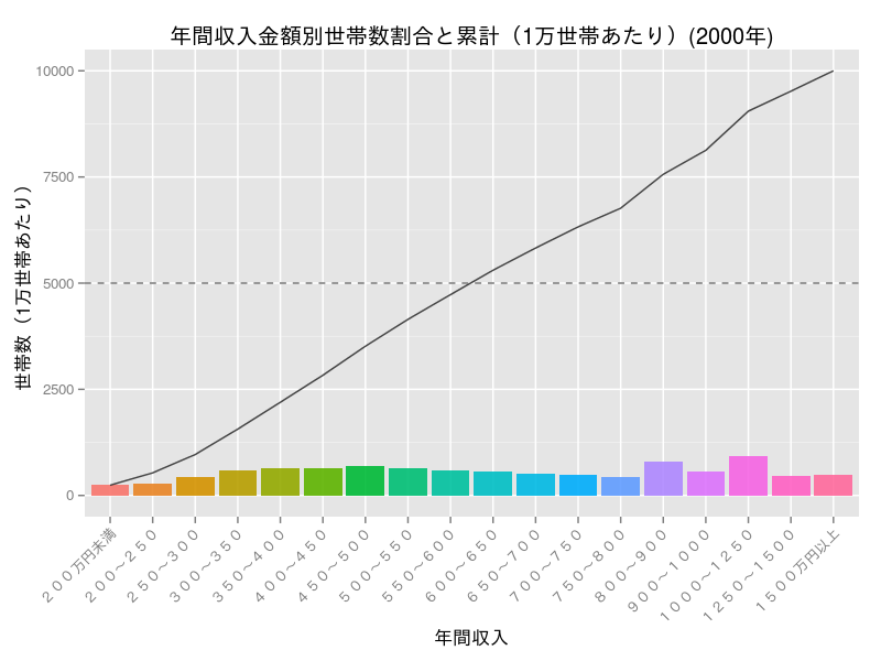
• 中央値約６００万円。第1四分位数約４００万円

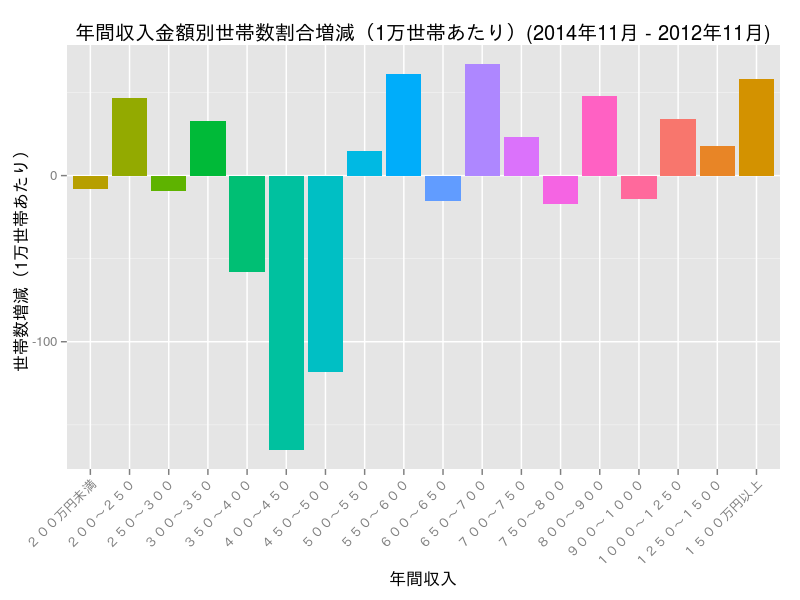
2014年11月と201２年11月年間収入金額別世帯数割合比較

家計調査 家計収支編 二人以上の世帯 詳細結果表 月次 2014年11月
平成26年(2014年)11月

variable<-c("２００万円未満","２００～２５０","２５０～３００","３００～３５０","３５０～４００","４００～４５０","４５０～５００","５００～５５０","５５０～６００","６００～６５０","６５０～７００","７００～７５０","７５０～８００","８００～９００","９００～１０００","１０００～１２５０","１２５０～１５００","１５００万円以上")
No<-c(1:18)
value<-c(246,497,665,947,866,791,661,747,631,525,536,421,343,578,394,579,264,310)
kakei<-data.frame(No,variable,value)
kakei$cumsum<-cumsum(kakei$value)
library(ggplot2)
ggplot(data=kakei)+
geom_bar(stat="identity", position = "dodge",aes(x=reorder(variable,No),y=value,group=variable,fill=variable),alpha=0.9)+
####ここから
#geom_hline(aes(yintercept=5000), colour="gray40", linetype="dashed",alpha=0.9)+
#geom_line(aes(x=No,y=cumsum),color="gray20",alpha=0.9)+
####ここまでコメントアウトすると棒グラフのみ
xlab("年間収入")+
ylab("世帯数（1万世帯あたり）")+
ggtitle("年間収入金額別世帯数割合と累計（1万世帯あたり）(2014年_11)") +
theme(legend.position = "no",axis.text.x = element_text(angle = 45, hjust = 1))
#ggsave("KRC2014_11.png",dpi = 100, width = 8, height = 6)

家計調査 家計収支編 二人以上の世帯 詳細結果表 月次 2012年11月
平成24年(2012年)11月

variable<-c("２００万円未満","２００～２５０","２５０～３００","３００～３５０","３５０～４００","４００～４５０","４５０～５００","５００～５５０","５５０～６００","６００～６５０","６５０～７００","７００～７５０","７５０～８００","８００～９００","９００～１０００","１０００～１２５０","１２５０～１５００","１５００万円以上")
No<-c(1:18)
value<-c(254,450,674,914,924,956,779,732,570,540,469,398,360,530,408,545,246,252)
kakei<-data.frame(No,variable,value)
kakei$cumsum<-cumsum(kakei$value)
library(ggplot2)
ggplot(data=kakei)+
geom_bar(stat="identity", position = "dodge",aes(x=reorder(variable,No),y=value,group=variable,fill=variable),alpha=0.9)+
####ここから
geom_hline(aes(yintercept=5000), colour="gray40", linetype="dashed",alpha=0.9)+
geom_line(aes(x=No,y=cumsum),color="gray20",alpha=0.9)+
####ここまでコメントアウトすると棒グラフのみ
xlab("年間収入")+
ylab("世帯数（1万世帯あたり）")+
ggtitle("年間収入金額別世帯数割合と累計（1万世帯あたり）(2012年_11)") +
theme(legend.position = "no",axis.text.x = element_text(angle = 45, hjust = 1))
#ggsave("KRC2012_11.png",dpi = 100, width = 8, height = 6)

階級別の増減を見るため、2014年11月のデータから2012年11月のデータをひいたデータを作成

value2014<-c(246,497,665,947,866,791,661,747,631,525,536,421,343,578,394,579,264,310)
value2012<-c(254,450,674,914,924,956,779,732,570,540,469,398,360,530,408,545,246,252)
value<-value2014-value2012
variable<-c("２００万円未満","２００～２５０","２５０～３００","３００～３５０","３５０～４００","４００～４５０","４５０～５００","５００～５５０","５５０～６００","６００～６５０","６５０～７００","７００～７５０","７５０～８００","８００～９００","９００～１０００","１０００～１２５０","１２５０～１５００","１５００万円以上")
No<-c(1:18)
kakei<-data.frame(No,variable,value)
ggplot(kakei, aes(x=reorder(variable,No),y=value)) + 
geom_bar(stat="identity", position = "dodge",aes(group=variable,fill=variable)) +
xlab("年間収入")+
ylab("世帯数増減（1万世帯あたり）")+
ggtitle("年間収入金額別世帯数割合増減（1万世帯あたり）(2014年11月 - 2012年11月)") +
theme(legend.position = "no",axis.text.x = element_text(angle = 45, hjust = 1))
#ggsave("KR201411_201211.png",dpi = 100, width = 8, height = 6)