平成28年10月21日鳥取県中部の地震4

raster , marmap , lattice , ggmap , xts パッケージ

(前の記事)
気象庁震源リスト03(熊本地震と新潟県中越地震)

四角で囲まれた部分の地形

中央の線部分の起伏

日別の地震

コードはほとんど過去の記事のどれかと同じ

1
2
3
4
5
6
7
8
9
10
11
12
13
14
15
16
library(raster)
library(rgdal)
#zipfile=tempfile()
#download.file("http://dds.cr.usgs.gov/srtm/version2_1/SRTM3/Eurasia/N35E133.hgt.zip",zipfile)
#unzip(zipfile)
t1 = raster('N35E133.hgt')
#download.file("http://dds.cr.usgs.gov/srtm/version2_1/SRTM3/Eurasia/N35E134.hgt.zip",zipfile)
#unzip(zipfile)
t2 = raster('N35E134.hgt')
#raster::merge関数はfilenameオプションで保存もできる
tottori<-merge(t1,t2)
slope <- terrain(tottori, opt='slope')
aspect <- terrain(tottori, opt='aspect')
hill <- hillShade(slope, aspect, 40, 270)
brks<-c(1,seq(100,2000,100))
arg <- list(at=c(0,500,1000,1500,2000), labels=c("0","500","1000","1500","2000"))
1
2
3
4
5
6
7
8
9
10
11
12
13
14
15
16
17
18
19
20
21
22
23
24
25
26
27
28
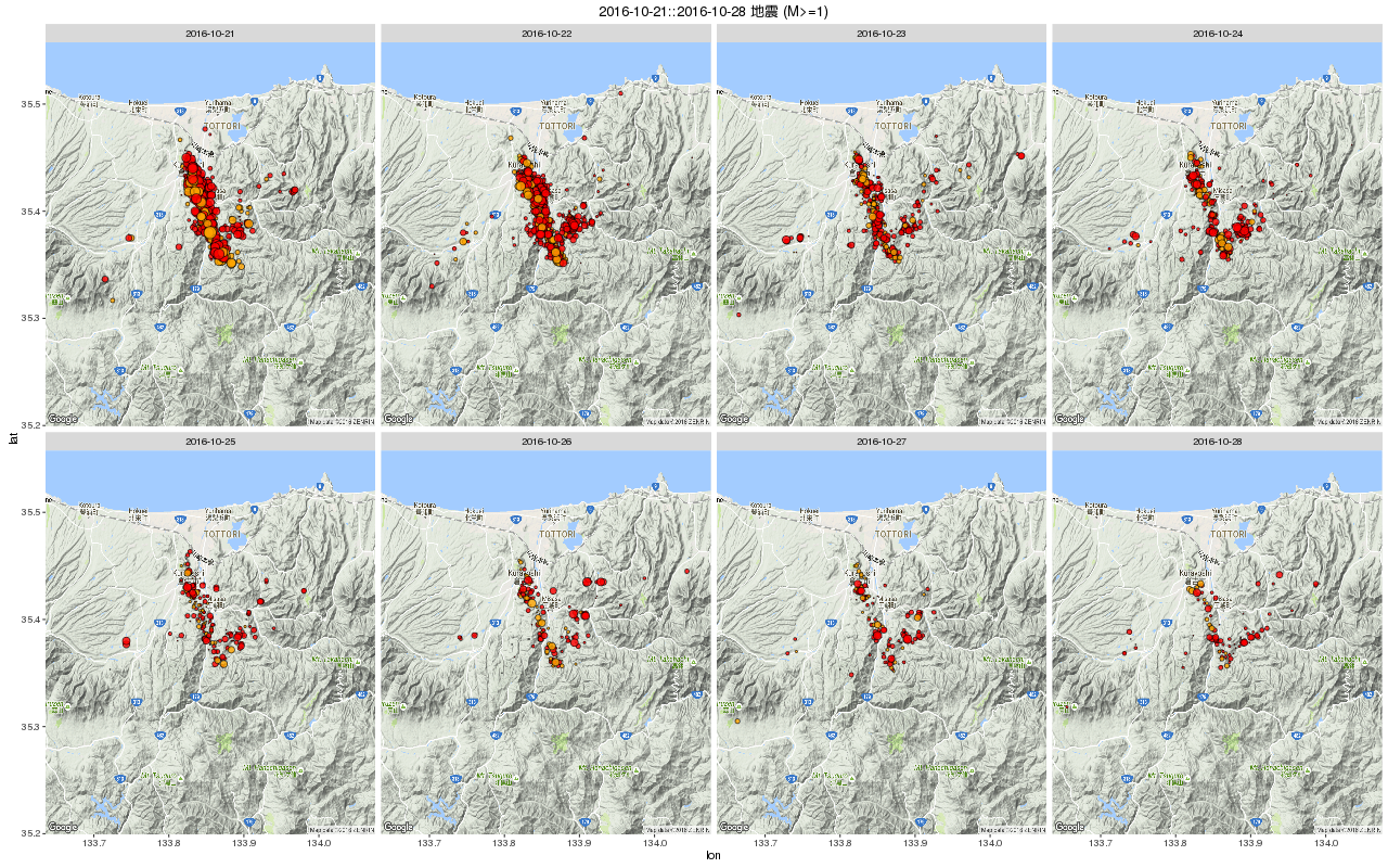
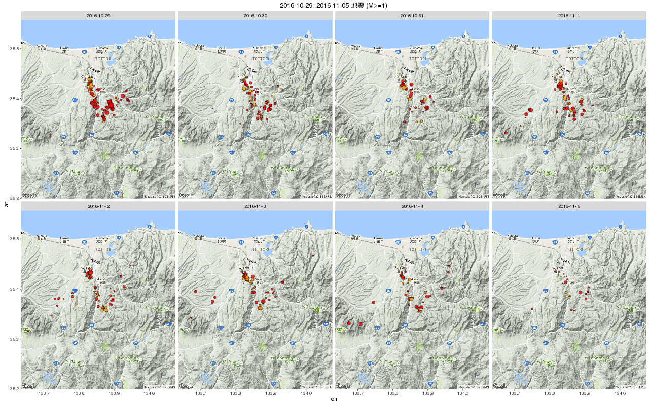
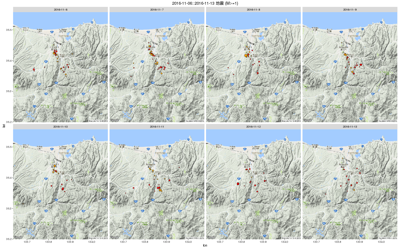
eqdata<-read.table(text="",col.names=c("time", "longitude", "latitude", "depth", "mag"))
ymd<-seq(as.Date("2016-10-21"),as.Date("2016-11-15"), by="1 day")
for (i in 1:length(ymd)){
date<-gsub("-","",ymd[i])
#ウェブスクレイピング
url<-paste0("http://www.data.jma.go.jp/svd/eqev/data/daily_map/",date,".html")
#
doc<-readLines(url,encoding ="UTF-8")
kensaku<-paste0(substr(date,1,4)," ",gsub("\\<0"," ",substr(date,5,6))," ",gsub("\\<0"," ",substr(date,7,8)))
#
x<-doc[grep(paste0("\\<",kensaku),doc)]
#全角文字 ° が入っているので半角スペース2つに変換する
x<-gsub("°", " ",x)
time<-paste0(substr(x,1,4),"-",substr(x,6,7),"-",substr(x,9,10)," ",substr(x,12,16),":",substr(x,18,21))
#
#南緯、西経の場合も考慮に入れると
latitude = as.numeric(paste0(substr(x,23,23),as.character(as.numeric(substr(x,24,25))+as.numeric(substr(x,28,29))/60+as.numeric(substr(x,31,31))/600)))
longitude = as.numeric(paste0(substr(x,34,34),as.character(as.numeric(substr(x,35,37))+as.numeric(substr(x,40,41))/60+as.numeric(substr(x,43,43))/600)))
depth<-as.numeric(substr(x,48,50))
mag<-as.numeric(substr(x,55,58))
eq<-data.frame(time,longitude,latitude,depth,mag)
eqdata<-rbind(eqdata,subset(eq,mag>=-4))
}
#
#重複した行を取り除く
eqdata<-unique(eqdata)
#head(eqdata) ; tail(eqdata)
#save(eqdata,file="eqdata20161021_1115.RData")
1
2
3
4
5
6
7
8
9
10
11
12
13
14
15
16
17
18
19
20
21
22
23
24
25
26
27
28
29
30
31
32
33
34
35
36
#load("eqdata20161021_1115.RData")
#震源の深さ
# depth<10km
eqdata1<-subset(eqdata,depth<10)
eqdata1$depth_rank<-" 10km 未満"
eqdata1$col<-"red"
# 10<=depth<20
eqdata2<-subset(eqdata,depth>=10 & depth<20)
eqdata2$depth_rank<-" 10km以上20km未満"
eqdata2$col<-"orange"
# 20<=depth<40
eqdata3<-subset(eqdata,depth>=20 & depth<40)
eqdata3$depth_rank<-" 20km以上40km未満"
eqdata3$col<-"gold4"
# 40<=depth<80
eqdata4<-subset(eqdata,depth>=40 & depth<80)
eqdata4$depth_rank<-" 40km以上80km未満"
eqdata4$col<-"green"
# 80<=depth<150
eqdata5<-subset(eqdata,depth>=80 & depth<150)
eqdata5$depth_rank<-" 80km以上150km未満"
eqdata5$col<-"blue"
# 150<=depth
eqdata6<-subset(eqdata,depth>=150)
eqdata6$depth_rank<-"150km以上"
eqdata6$col<-"purple"
#
eq<-rbind(eqdata1,eqdata2,eqdata3,eqdata4,eqdata5,eqdata6)
#並べ替え:マグニチュードの昇順
sortlist <- order(eq$mag)
eq<- eq[sortlist,]
##
#mag>=1の地震を抽出
subeq<-subset(eq,mag>=1)
#mag<1
mag1und<-subset(eq,mag<1)
1
2
3
4
5
6
7
8
9
10
11
12
13
14
15
16
17
18
19
20
21
22
23
24
25
26
27
28
29
30
31
32
33
34
35
36
Crop <- c(133.18,134.42,35,35.7)
tottori_crop <- crop(tottori,Crop)
slope_crop <- terrain(tottori_crop, opt='slope')
aspect_crop <- terrain(tottori_crop, opt='aspect')
hill_crop <- hillShade(slope_crop, aspect_crop, 40, 270)
#
#png("tyubu1021_1115.png",width=800,height=600)
plot(hill_crop, col=grey(0:100/100), legend=FALSE, main="",las=1)
plot(tottori_crop,breaks=brks,col=terrain.colors(25,alpha=0.35), add=TRUE, axis.args=arg)
#
points(x=mag1und$longitude, y=mag1und$latitude,cex=0.2,pch=21,bg=mag1und$col,col=mag1und$col)
points(x=subeq$longitude, y=subeq$latitude,cex=subeq$mag/2,pch=21,bg=subeq$col,col="gray20")
par(xpd=T)
#
#par("usr")[1]~par("usr")[4] : x軸の最小値,最大値, y軸の最小値,最大値
#
cexsize=c(1,3,5,7)/2
#
#legend(par("usr")[1]*0.08+par("usr")[2]*0.92,par("usr")[3]*0.5+par("usr")[4]*0.5,title="Magnitude",
#legend = c("M=1","M=3","M=5","M=7"), col=1,pch=21,pt.cex=cexsize,
#cex =1,bg ="gray90", x.intersp = 2, y.intersp =1.65,bty = "o")
#
#legend(par("usr")[1]*0.08+par("usr")[2]*0.92,par("usr")[3]*0.45+par("usr")[4]*0.55,title="Magnitude",
legend("right",par("usr")[3]*0.3+par("usr")[4]*0.7,title="Magnitude",
legend = c("M<1","M=1","M=3","M=5","M=7"), col=1,pch=21,pt.cex=c(0.2,cexsize),
cex =1,bg ="gray90", x.intersp = 2, y.intersp =1.65,bty = "o")
#
#legend(par("usr")[1]*0.15+par("usr")[2]*0.85,par("usr")[3]*0.75+par("usr")[4]*0.25,title="Depth",
legend("bottomright",title="Depth",
legend = c("D<10km","10km<=D<20km","20km<=D<40km","40km<=D<80km","80km<=D<150km","150km<=D"),
cex=1,pch=19,col=c("red","orange","gold4","green","blue","purple"),
pt.cex =1.5,bg ="gray90", x.intersp = 1, y.intersp =1.2,bty = "o")
par(xpd=F)
title(paste0(ymd[1],"~",ymd[length(ymd)]," 地震")) # (mag>=1)
title("","( データ:気象庁 震源リスト )",line=2)
#dev.off()
1
2
3
4
5
6
7
8
9
10
11
library(marmap)
tmar <- as.bathy(tottori_crop)
#
#png("tyubu1021_1115_05.png",width=800,height=600)
plot(tmar,land=TRUE,col=rgb(0,0,0,0.5))
points(x=mag1und$longitude, y=mag1und$latitude,cex=0.2,pch=21,bg=mag1und$col,col=mag1und$col)
points(x=subeq$longitude, y=subeq$latitude,cex=subeq$mag/2,pch=21,bg=subeq$col,col="gray20")
#
belt <- get.box(tmar, x1 = 133.82, x2 = 133.88, y1 = 35.475, y2 = 35.338,
col = "blue",lwd=1.5,width = 0.1)
#dev.off()
1
2
3
4
5
6
7
8
library(lattice)
#png("tyubu1021_1115_06.png",width=800,height=600)
wireframe(belt, shade = TRUE, zoom = 1.1,
aspect = c(1/4, 0.1),
screen = list(z = -60, x = -60),
par.settings = list(axis.line = list(col = "transparent")),
par.box = c(col = rgb(0, 0, 0, 0.5)))
#dev.off()
1
2
3
4
5
trsect <- get.transect(tmar, 133.82, 35.475, 133.88, 35.338, distance = TRUE)
#head(trsect)
#png("tyubu1021_1115_07.png",width=800,height=600)
plotProfile(trsect)
#dev.off()
1
2
3
4
5
6
7
8
9
10
11
12
13
14
15
16
17
18
19
20
21
22
23
24
25
26
27
28
29
30
31
32
33
34
35
36
37
38
39
40
41
42
43
44
45
46
47
48
49
50
library(ggmap)
library(ggplot2)
library(xts)
#
gmap <- get_map(c(133.855,35.379),zoom = 11, maptype = "terrain")
attr(gmap,"b")
#
# 1時間ごと
# 1時間ごとにプロットする準備
#eq$period<-substring(eq$time,1,13)
# 1日ごと
# 1日ごとにプロットする準備
eq$period<-substring(eq$time,1,10)
#subeq$period<-substring(subeq$time,1,10)
#プロットする期間を抽出する場合
#時間単位で取り出す場合 xts(eq[,-1], as.POSIXct(eq$time)) とする
eq.xts<-xts(eq[,-1], as.POSIXct(eq$time))
#
# 2016-10-21::2016-10-28の場合
days<-"2016-10-21::2016-10-28"
subeq<-data.frame(coredata(eq.xts[days]),stringsAsFactors = F)
#str(subeq)
#文字列になってしまったところをnumericに変換
subeq<-transform(subeq,longitude = as.numeric(longitude),latitude= as.numeric(latitude),depth= as.numeric(depth),mag= as.numeric(mag))
#マグニチュードの昇順に並べ替え
sortlist <- order(subeq$mag)
subeq<- subeq[sortlist,]
#
### マグニチュード1以上の地震をプロット
#mag>=1の地震を抽出
subeq<-subset(subeq,mag>=1)
#
lon1=c(attr(gmap,"b")$ll.lon,attr(gmap,"b")$ur.lon)
lat1=c(attr(gmap,"b")$ll.lat,attr(gmap,"b")$ur.lat)
#
p<-ggmap(gmap)+
#指定した範囲きっかりに描画
coord_cartesian(xlim=c(lon1[1],lon1[2]),ylim=c(lat1[1],lat1[2])) +
geom_point(data=subeq, aes(x=longitude, y=latitude,fill=depth_rank,size=mag),alpha=0.8,shape=21,color="black")+
#プロットする色を指定したい場合
scale_fill_manual(values=c("red","orange","gold4","green","blue","purple"),
breaks = c(" 10km 未満"," 10km以上20km未満"," 20km以上40km未満"," 40km以上80km未満"," 80km以上150km未満","150km以上"))+
#プロットする大きさの範囲を指定したい場合
scale_size(breaks=c(1,3,5,7),range = c(0.1,5))+
guides(fill=FALSE , size=FALSE)
#
#2016-10-21::2016-10-28の場合
#png("tyubu1021_1115_02.png",width=1280,height=800)
p+facet_wrap(~period,ncol=4) + labs(title=paste0(days," 地震 (M>=1)"))
#dev.off()