海底地形と地形データ02

raster , marmap , rgdal , geosphere パッケージ

(前の記事)
マグニチュード6以上
海底地形と地形データ

(参考)
(参考 : データの引用文献等)
関東地震,東海地域のアスペリティ,東海・東南海・南海地震の想定震源域
駿河トラフ,相模トラフ,南海トラフ

Fuyuki Hirose’s HP
プレート形状の数値データ

出典論文

東北地方南部~関東地方
Nakajima and Hasegawa (2006, GRL),弘瀬・他 (2008, 地震),Nakajima et al. (2009, JGR)

西南日本
Baba et al. (2002, PEPI),Nakajima and Hasegawa (2007, JGR),Hirose et al. (2008, JGR)

(準備)

  • 関東地震,東海地域のアスペリティ,東海・東南海・南海地震の想定震源域
    駿河トラフ,相模トラフ,南海トラフにヘッダーを加えて、csvファイルに変換した。
  • 気象庁の地震カタログ、震源リストからデータをダウンロード、加工、日本周辺で起きたマグニチュード6以上データを抽出。

今回はggplot2パッケージを使いません。

1
2
3
4
5
6
7
8
9
10
11
12
13
14
15
16
17
18
19
20
21
22
23
24
25
26
27
28
29
30
31
32
33
34
35
36
37
library(marmap)
library(rgdal)
library(raster)
Lon.range = c(122, 154)
Lat.range = c(20, 46)
dat<-getNOAA.bathy(Lon.range[1],Lon.range[2],Lat.range[1],Lat.range[2],res=4,keep=TRUE)
#
r1<-marmap::as.raster(dat)
#配色はGMTのカラーパレット“relief”を参考にした
oce<-colorRampPalette(c(rgb(0,0,0),rgb(0,5/255,25/255),rgb(0,10/255,50/255),rgb(0,80/255,125/255),rgb(0,150/255,200/255),
rgb(86/255,197/255,184/255),rgb(172/255,245/255,168/255),rgb(211/255,250/255,211/255),rgb(1,1,1)))
#
land1 <- colorRampPalette(c("#467832","#786432"))
land2 <- colorRampPalette(c("#786432","#927E3C"))
land3 <- colorRampPalette(c("#927E3C","#C6B250"))
land4 <- colorRampPalette(c("#C6B250","#FAE664"))
land5 <- colorRampPalette(c("#FAE664","#FAEA7E"))
breakpoints <- c(seq(-10000,0,10000/100),1 ,seq(50,500,50),seq(550,1000,50),seq(1100,2000,100),seq(2100,3000,100),seq(3500,8000,500))
colors <- c(oce(100),rgb(70/255,120/255,50/255),land1(10),land2(10),land3(10),land4(10),land5(10))
#
#plot(r1,breaks=breakpoints,col=colors)
#
#plot(r1,breaks=breakpoints,col=colors, axis.args=list(at=c(-8000,-4000,0,4000,8000), labels=c(-8000,-4000,0,4000,8000)),
# legend.args=list(text=" height (m)", side=3, font=2, line=1.5, cex=0.8),las=1)
#
#png("noaa01.png",width=600,height=600)
plot(r1,breaks=breakpoints,col=colors, axis.args=list(at=c(-8000,-4000,0,4000,8000), labels=c(-8000,-4000,0,4000,8000)),
legend.args=list(text=" height (m)", side=3, font=2, line=1.5, cex=0.8),las=1,axes=F,box=F)
par(xpd=T)
axes1<-seq(125,150,5)
axes2<-seq(20,45,5)
text(axes1,Lat.range[1],as.character(axes1),pos=1)
text(Lon.range[1],axes2,as.character(axes2),pos=2)
rect(Lon.range[1],Lat.range[1],Lon.range[2],Lat.range[2])
par(xpd=F)
title("Map")
#dev.off()

1
2
3
4
5
6
7
8
#png("noaa02.png",width=600,height=600)
slope <- terrain(r1, opt='slope')
aspect <- terrain(r1, opt='aspect')
hill <- hillShade(slope, aspect, 40, 270)
#png("r1001.png",width=1000,height=1000)
plot(hill, col=grey(0:100/100), legend=FALSE, main='map')
plot(r1,breaks=breakpoints,col=colors,alpha=0.35, add=TRUE, axis.args=list(at=c(-8000,-4000,0,4000,8000), labels=c(-8000,-4000,0,4000,8000)))
#dev.off()

1
2
3
4
5
6
7
8
9
10
11
12
13
14
15
16
17
18
19
20
21
22
23
24
25
26
27
28
29
30
31
32
33
34
35
36
37
38
39
40
41
42
43
44
45
46
47
48
49
50
51
52
53
54
55
56
57
58
59
60
61
62
63
64
65
66
67
68
69
70
71
72
73
74
75
76
77
78
79
80
81
82
83
84
85
86
87
88
89
90
91
92
93
94
95
96
97
98
99
100
101
102
103
104
105
106
107
108
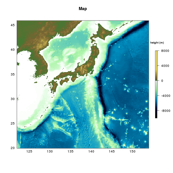
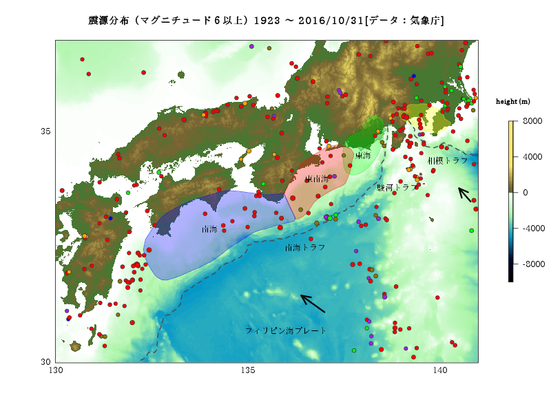
load("eq61923_20161031.RData")
eqdata<-eq6
#震源の深さ
# depth<10km
eqdata1<-subset(eqdata,depth<10)
eqdata1$depth_rank<-" 10km 未満"
eqdata1$col<-"red"
# 10<=depth<20
eqdata2<-subset(eqdata,depth>=10 & depth<20)
eqdata2$depth_rank<-" 10km以上20km未満"
eqdata2$col<-"orange"
# 20<=depth<40
eqdata3<-subset(eqdata,depth>=20 & depth<40)
eqdata3$depth_rank<-" 20km以上40km未満"
eqdata3$col<-"gold4"
# 40<=depth<80
eqdata4<-subset(eqdata,depth>=40 & depth<80)
eqdata4$depth_rank<-" 40km以上80km未満"
eqdata4$col<-"green"
# 80<=depth<150
eqdata5<-subset(eqdata,depth>=80 & depth<150)
eqdata5$depth_rank<-" 80km以上150km未満"
eqdata5$col<-"blue"
# 150<=depth
eqdata6<-subset(eqdata,depth>=150)
eqdata6$depth_rank<-"150km以上"
eqdata6$col<-"purple"
#
eq<-rbind(eqdata1,eqdata2,eqdata3,eqdata4,eqdata5,eqdata6)
#並べ替え:マグニチュードの昇順
sortlist <- order(eq$mag)
eq<- eq[sortlist,]
##
tokai=read.csv("./mapdata/tokai.csv")
tonankai=read.csv("./mapdata/tonankai.csv")
nankai=read.csv("./mapdata/nankai.csv")
# Asperities
# Kanto (Wald and Somerville, 1995, BSSA)
kasp=read.csv("./mapdata/kanto_eq.csv")
# Tokai (Matsumura, 1997, Tectono.)
tasp=read.csv("./mapdata/tokai_asperity.csv")
#
trench=read.csv("./mapdata/trench.csv")
#voldata=read.csv("./mapdata/voldata.csv")
#
trough<-data.frame(names=c("駿河トラフ","相模トラフ","南海トラフ","フィリピン海プレート","東海","東南海","南海"),
longitude=c(138.9,140.2,136.5,136,138,136.8,134),latitude=c(33.8,34.4,32.5,30.7,34.5,34,32.9))
#
library(marmap)
library(rgdal)
library(raster)
library("geosphere")
Lon.range = c(130, 141)
Lat.range = c(30, 37)
dat<-getNOAA.bathy(Lon.range[1],Lon.range[2],Lat.range[1],Lat.range[2],res=1,keep=TRUE)
#
r1<-marmap::as.raster(dat)
# 配色はGMTのカラーパレット“relief”を参考にした
oce<-colorRampPalette(c(rgb(0,0,0),rgb(0,5/255,25/255),rgb(0,10/255,50/255),rgb(0,80/255,125/255),rgb(0,150/255,200/255),
rgb(86/255,197/255,184/255),rgb(172/255,245/255,168/255),rgb(211/255,250/255,211/255),rgb(1,1,1)))
#
land1 <- colorRampPalette(c("#467832","#786432"))
land2 <- colorRampPalette(c("#786432","#927E3C"))
land3 <- colorRampPalette(c("#927E3C","#C6B250"))
land4 <- colorRampPalette(c("#C6B250","#FAE664"))
land5 <- colorRampPalette(c("#FAE664","#FAEA7E"))
breakpoints <- c(seq(-10000,0,10000/100),1 ,seq(50,500,50),seq(550,1000,50),seq(1100,2000,100),seq(2100,3000,100),seq(3500,8000,500))
colors <- c(oce(100),rgb(70/255,120/255,50/255),land1(10),land2(10),land3(10),land4(10),land5(10))
#
#plot(r1,breaks=breakpoints,col=colors)
#
#plot(r1,breaks=breakpoints,col=colors, axis.args=list(at=c(-8000,-4000,0,4000,8000), labels=c(-8000,-4000,0,4000,8000)),
# legend.args=list(text=" height (m)", side=3, font=2, line=1.5, cex=0.8),las=1)
#
#png("noaa1923_2016.png",width=800,height=600)
par(family="TakaoExMincho")
plot(r1,breaks=breakpoints,col=colors, axis.args=list(at=c(-8000,-4000,0,4000,8000), labels=c(-8000,-4000,0,4000,8000)),
legend.args=list(text=" height (m)", side=3, font=2, line=1.5, cex=0.8),las=1,axes=F,box=F)
par(xpd=T)
axes1<-seq(130,140,5)
axes2<-seq(30,35,5)
text(axes1,Lat.range[1],as.character(axes1),pos=1)
text(Lon.range[1],axes2,as.character(axes2),pos=2)
rect(Lon.range[1],Lat.range[1],Lon.range[2],Lat.range[2])
par(xpd=F)
title("震源分布(マグニチュード6以上)1923 ~ 2016/10/31[データ:気象庁]")
#
polygon(x=tokai$longitude, y = tokai$latitude, col=rgb(0,1,0,0.3),border=rgb(0,1,0,0.5))
polygon(x=tonankai$longitude, y = tonankai$latitude,col=rgb(1,0,0,0.3),border=rgb(1,0,0,0.5))
polygon(x=nankai$longitude, y = nankai$latitude, col=rgb(0,0,1,0.3),border=rgb(0,0,1,0.5))
#
polygon(x=kasp$longitude, y = kasp$latitude,col=rgb(1,1,0,0.3),border=rgb(1,1,0,0.5))
polygon(x=tasp$longitude, y = tasp$latitude,col=rgb(0,0.5,0,0.3),border=rgb(0,0.5,0,0.5))
#
trench1=trench[trench$latitude>=30 & trench$longitude<=141,]
lines(x=trench1$longitude, y = trench1$latitude,col="gray30",lty=2,lwd=2)
#
eq1=eq[eq$longitude>=130 & eq$longitude<=141 & eq$latitude>=30 & eq$latitude<=37,]
points(x=eq1$longitude, y=eq1$latitude,cex=eq1$mag/6,pch=21,bg=eq1$col,col="gray20")
#
text(x = trough$longitude, y = trough$latitude,labels =trough$names)
#
arrow1<-destPointRhumb(c(140.8,33.5),90-131, 63750/3*2)
arrow2<-destPointRhumb(c(137,31.1),90-145, 105000/3*2)
arrows(140.8,33.5,arrow1[1],arrow1[2],angle = 25, length = 0.2, code = 2,lwd=3)
arrows(137,31.1,arrow2[1],arrow2[2],angle = 25, length = 0.2, code = 2,lwd=3)
#
#dev.off()