日銀買入額(2010-12-15~2016-02-19)

ggplot2,xts,quantmod,gdata パッケージ

(過去の記事)
日銀買入額
日銀買入額(2010-12-15~2015-07-09)

使用したデータ
http://www3.boj.or.jp/market/jp/pastetfreit.zip

上のデータから作成したデータファイル:2010_2015 (コードの中で読み込む)

d2010_2015.RData

コードの中で読み込むデータ:2016年分
http://www3.boj.or.jp/market/jp/etfreit.zip

1
2
3
4
5
6
7
8
9
10
11
12
13
14
15
16
17
18
19
20
21
22
23
24
25
26
27
28
29
30
31
32
33
34
35
36
37
38
39
40
41
42
43
44
45
46
library(xts)
library(gdata)
library(ggplot2)
library(grid)
library(quantmod)
library(ggthemes)
#
#作成したデータファイル読み込み
load(url("http://statrstart.github.io/data/d2010_2015.RData"))
#
#日銀のサイトからデータを取り込む
temp <- tempfile()
download.file("http://www3.boj.or.jp/market/jp/etfreit.zip",temp)
con <- unzip(temp, "2016.xls")
d2016 <- read.xls(con,header=F,skip=8)
unlink(temp)
d2016<-d2016[,2:4]
names(d2016)<-c("date","ETF","REIT")
d2016$ETF[is.na(d2016$ETF)]<-0
d2016$REIT[is.na(d2016$REIT)]<-0
#rbind
d2010_2016<-rbind(d2010_2015,d2016)
#
x <- read.zoo(d2010_2016)
#
#ggplot(aes(x = Index, y = Value,group=Series,fill=Series), data = fortify(x, melt = TRUE)) +
#geom_bar(stat="identity",position=position_dodge()) +
#facet_wrap(~ Series,nrow=2)+
#labs(title="日銀買い入れ", x="", y="")+
#guides(fill=FALSE)
#
#
#ETF
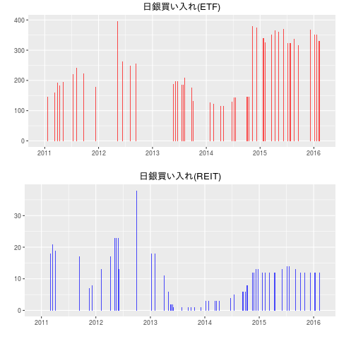
a<-ggplot(data = fortify(x[,1], melt = TRUE),aes(x = Index, y = Value) ) +
geom_bar(stat="identity",position=position_dodge(),fill=rgb(1,0,0,alpha=0.7)) +
labs(title="日銀買い入れ(ETF)", x="", y="")
#REUT
b<-ggplot(data = fortify(x[,2], melt = TRUE),aes(x = Index, y = Value) ) +
geom_bar(stat="identity",position=position_dodge(),fill=rgb(0,0,1,alpha=0.7)) +
labs(title="日銀買い入れ(REIT)", x="", y="")
#png("boj20160219_1.png")
grid.newpage() #空の画面を作る
pushViewport(viewport(layout=grid.layout(2, 1))) #画面を区切る
print(a, vp=viewport(layout.pos.row=1))
print(b, vp=viewport(layout.pos.row=2))
#dev.off()

heatmap

1
2
3
4
5
6
7
8
9
10
#devtools::install_github("Ather-Energy/ggTimeSeries")
library(ggTimeSeries)
library(data.table)
d2010_2016$date<-as.Date(d2010_2016$date)
d2010_2016<-setDT(d2010_2016)
#png("boj20160219_3.png")
p1<-ggplot_calendar_heatmap(d2010_2016,"date","ETF")
p1 + xlab('') + ylab('') + scale_fill_continuous(low = 'green', high = 'red') +
facet_wrap(~Year, ncol = 1)
#dev.off()

累計

1
2
3
4
5
6
7
8
9
10
11
12
13
14
#ETF累計
a<-ggplot(data = fortify(cumsum(x[,1]), melt = TRUE),aes(x = Index, y = Value) ) +
geom_bar(stat="identity",position=position_dodge(),fill=rgb(1,0,0,alpha=0.7)) +
labs(title="日銀買い入れ:累計(ETF)", x="", y="")
#REIT累計
b<-ggplot(data = fortify(cumsum(x[,2]), melt = TRUE),aes(x = Index, y = Value) ) +
geom_bar(stat="identity",position=position_dodge(),fill=rgb(0,0,1,alpha=0.7)) +
labs(title="日銀買い入れ:累計(REIT)", x="", y="")
#png("boj20160219_2.png")
grid.newpage() #空の画面を作る
pushViewport(viewport(layout=grid.layout(2, 1))) #画面を区切る
print(a, vp=viewport(layout.pos.row=1))
print(b, vp=viewport(layout.pos.row=2))
#dev.off()

  • こんなに増やして売るときどうするの? どうなるの?

日経平均株価

1
2
3
4
5
6
getSymbols('^N225',from ="2010-12-15")
#png("N225boj.png")
n225<-autoplot(N225$N225.Close)+labs(title="N225.Close")
n225 + theme_economist()
#+ scale_colour_economist()
#dev.off()

買入日の株価指数の終値でETF(日経平均株価)の買入を行ったと仮定すると、

1
2
3
d2010_2016<-setDF(d2010_2016)
dat<-merge(d2010_2016,data.frame(date=index(N225),coredata(N225$N225.Close)))
sum(dat$ETF)/sum(dat$ETF/dat$N225.Close)
14452.49 (受け取った配当等は加味していません)

「日銀 含み損」や「日銀 ETF 簿価」をキーワードとしてググると、もっと詳しく試算しているサイトがある。

試算ではないけれどこんなレポートをみつけた。
公的機関の株式保有動向(2015年11月10日)