ランドサット8号のデータ5(一連の操作)

rLandsat8 , RStoolbox , raster , colorRamps パッケージ

(参考)
Using the USGS Landsat 8 Product
rLandsat8 - an R interface to Landsat8
RStoolbox::panSharpen.R

データはLandBrowserより

操作1(必要な部分を切り出し。可視光の画像を作成。)

関数を読み込む
1
2
3
4
5
6
7
8
9
10
11
12
13
14
15
16
17
18
19
20
21
22
23
24
25
26
#付け加えた関数(landsat8のメタファイル(ファイル名の後ろが"_MTL.txt")を読み込む)
read.meta<- function(product){
meta.file <- paste0(product, "/", product, "_MTL.txt")
textLines <- readLines(meta.file)
met <- read.table(text=textLines[grep("=", textLines)],header = FALSE, sep = "=", strip.white = TRUE,
stringsAsFactors = FALSE,row.names = NULL, col.names = c("name", "value"))
met <- met[!met$name == "GROUP", ]
met <- met[!met$name == "END_GROUP", ]
rownames(met) <- tolower(met[, "name"])
met[, "name"] <- NULL
met <- as.list(as.data.frame(t(met), stringsAsFactors = FALSE))
return(met)
}
##環境によってはRStoolboxパッケージがインストールできないのでpanSharpenのみ取り出し。
#使う方法は method = "brovey"だけにした。
panSharpen <- function(img, pan, r, g, b) {
stopifnot(inherits(img, "Raster") & inherits(pan, "Raster"))
layernames <- names(img)[c(r,g,b)]
ordr <- match(layernames, names(img))
layernames <- layernames[order(ordr)]
msi <- resample(img[[layernames]], pan, method = "ngb")
mult <- pan / sum(msi)
panimg <- msi * mult
names(panimg) <- paste0(layernames, "_pan")
panimg
}

データは/home/user/landsat8内のフォルダに置く

不要な部分は行頭に#をつけ、必要なら#をとる。

(例)阿蘇山の部分を切り出し。可視光の画像を作成。

2015年1月13日のデータです。

1
2
3
4
5
6
7
8
9
10
11
12
13
14
15
16
17
18
19
20
21
22
23
24
25
26
27
28
29
30
31
32
33
34
35
36
37
38
39
40
41
42
43
44
45
46
47
48
49
50
51
52
53
54
55
56
57
58
59
60
61
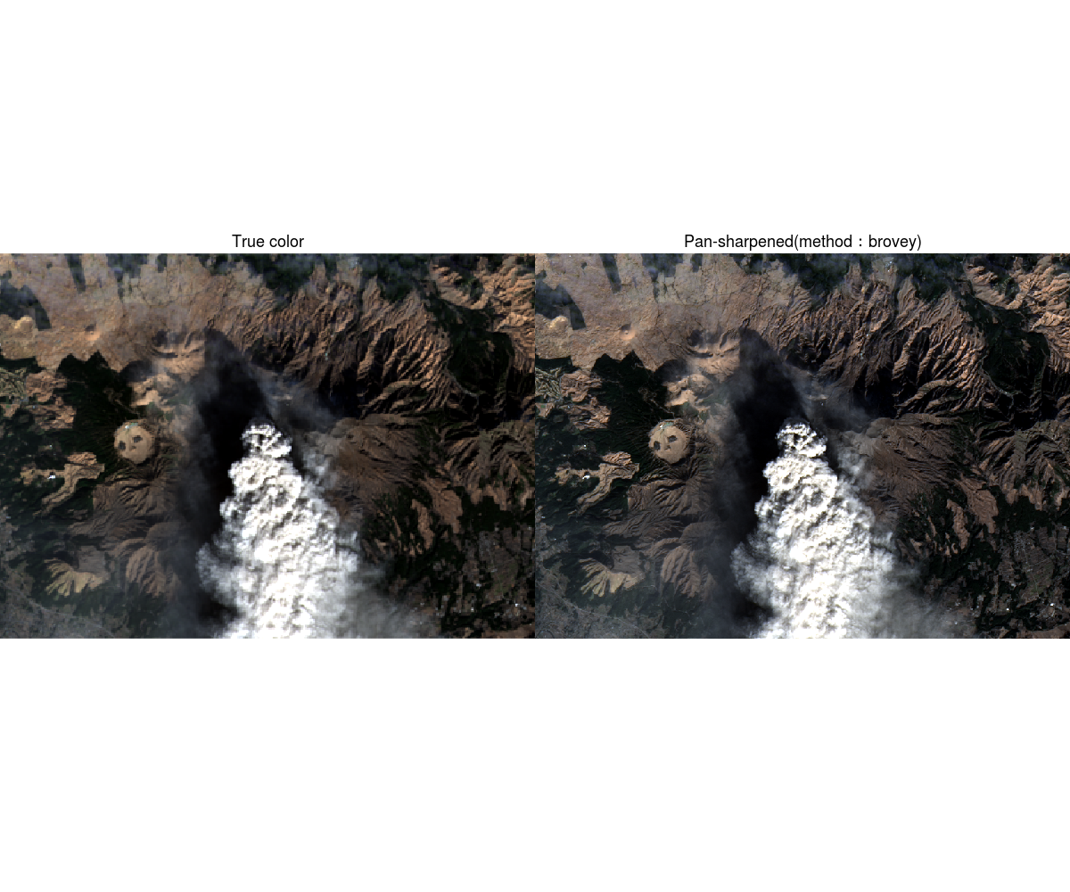
library(raster)
library(colorRamps)
library(RColorBrewer)
#library(devtools)
#install_url("https://github.com/Terradue/rLandsat8/releases/download/v0.1-SNAPSHOT/rLandsat8_0.1.0.tar.gz")
library(rLandsat8)
#source("rLandsat8fix.R") #変更した関数付け加えた関数をrLandsat8fix.Rというファイル名で作業フォルダに保存した場合。
setwd("/home/user/landsat8")
#阿蘇山 path:112 row:037
product <- "LC81120372015013LGN00"
Crop <- c(689000,701500,3635500,3644500)
fname0<-"aso"
#西之島 path:105 row:041
#product <- "LC81050412015172LGN00"
#Crop<-c(485700,491000,3011000,3016000)
#fname0<-"nishinoshima"
#鳥取市 path:111 row:035
#product <- "LC81110352015214LGN00"
#Crop <- c(420000,430000,3926000,3934600)
#fname0<-"tottori"
#福島 path:107 row:034
#product <- "LC81070342015218LGN00"
#Crop<-c(490000,512000,4125000,4150000)
#fname0<-"fukushima"
#桜島 path:112 row:038
#product <- "LC81120382015221LGN00"
#Crop <- c(650700,664300,3490800,3501200)
#fname0<-"sakurazhima"
#メタデータの読み込み
meta<-read.meta(product)
date<-meta$date_acquired
#保存するファイル名,作成する画像のファイル名の基礎
fname<-paste0(fname0,substr(date,1,4),substr(date,6,7),substr(date,9,10))
#解像度=30m
OLI<-stack(c(aerosol=paste0(product,"/",product, "_B1.TIF"),blue=paste0(product,"/",product, "_B2.TIF"),
green=paste0(product,"/",product, "_B3.TIF"),red=paste0(product,"/",product, "_B4.TIF"),
nir=paste0(product,"/",product, "_B5.TIF"),swir1=paste0(product,"/",product, "_B6.TIF"),
swir2=paste0(product,"/",product, "_B7.TIF"),cirrus=paste0(product,"/",product, "_B9.TIF")))
#解像度=15m
PAN <-stack(paste0(product,"/",product, "_B8.TIF"))
names(PAN)<-"panchromatic"
#解像度=100m
TIRS<-stack(c(tirs1=paste0(product,"/",product, "_B10.TIF"),tirs2=paste0(product,"/",product, "_B11.TIF")))
#必要な部分の切り出し
subOLI <- crop(OLI,Crop)
subPAN <- crop(PAN,Crop)
subTIRS <- crop(TIRS,Crop)
#library(devtools)
#install_github("bleutner/RStoolbox")
#library(RStoolbox)
## Brovey pan sharpening
RGBpan <- panSharpen(subOLI,subPAN, r = 4, g = 3, b = 2)
## Plot
#png(paste0(fname,"_1.png"),width=1200,height=1000)
par(mfrow=c(1,2))
plotRGB(subOLI, r = 4, g = 3, b = 2, stretch = "lin")
text((Crop[1]+Crop[2])/2,Crop[4],"True color",pos=3, cex=1.5)
plotRGB(RGBpan,r = 3, g = 2, b = 1,stretch="lin")
text((Crop[1]+Crop[2])/2,Crop[4],"Pan-sharpened(method:brovey)",pos=3, cex=1.5)
par(mfrow=c(1,1))
#dev.off()

操作2(メタデータと切り出し部分をリスト化。必要なら保存。)

1
2
3
4
5
bands=c(unstack(subOLI)[1:7],unstack(subPAN),unstack(subOLI)[8],unstack(subTIRS))
l<-list(metadata = meta, band = bands)
names(l$band)<-c("aerosol","blue", "green", "red","nir","swir1","swir2","panchromatic","cirrus","tirs1","tirs2")
#保存する場合は#をとる。
#save(l,file=paste0(fname,"_1.RData"))

操作3(輝度温度,正規化植生指数等の計算、図化)

パッケージと関数を読み込む
1
2
3
4
5
6
7
8
9
10
11
12
13
14
15
16
17
18
19
20
21
22
23
24
25
26
27
28
29
30
library(raster)
library(colorRamps)
#library(RColorBrewer)
library(rLandsat8)
#反射率(Reflectance)
#太陽天頂角を考慮する(変更後)
ToTOAReflectance <- function(landsat8, band) {
bandnames <- c("aerosol", "blue", "green", "red", "nir",
"swir1", "swir2", "panchromatic", "cirrus", "tirs1",
"tirs2")
idx <- seq_along(bandnames)[sapply(bandnames, function(x) band %in%
x)]
ml <- as.numeric(landsat8$metadata[[paste0("reflectance_mult_band_",
idx)]])
al <- as.numeric(landsat8$metadata[[paste0("reflectance_add_band_",
idx)]])
# TOAref <- landsat8$band[[band]] * ml + al
TOAref <- (landsat8$band[[band]] * ml + al)/sin(as.numeric(landsat8$metadata$sun_elevation) * pi /180)
return(TOAref)
}
#改良型正規化水指数(MNDWI)
#greenがgreebになっていたのを直した。
ToMNDWI <- function(landsat8) {
# MNDWI=(Green - SWIR1)/(Green + SWIR1)
green <- ToTOAReflectance(landsat8, "green")
swir1 <- ToTOAReflectance(landsat8, "swir1")
# mndwi <- (greeb - swir1)/(green + swir1)
mndwi <- (green - swir1) / (green + swir1)
return(mndwi)
}
計算と図化
1
2
3
4
5
6
7
8
9
10
11
12
13
14
15
16
17
18
19
20
21
22
23
24
25
26
27
28
29
30
31
32
33
34
35
36
37
38
39
40
41
42
43
#setwd("/home/user/landsat8")
#load(paste0(fname,"_1.RData")) #保存したデータ名
##放射輝度(Radiance)
#ToTOARadiance(landsat8=l, band="blue")
#太陽天頂角を考慮した反射率(Reflectance)(変更後)
#sin(as.numeric(l$metadata$sun_elevation) * pi /180)
#0.8912265 <-この数で割る。
#ToTOAReflectance(landsat8=l, band="blue")
#スペクトル放射輝度から温度(btemp: 絶対温度(K))
btemp <- ToAtSatelliteBrightnessTemperature(l, band="tirs1")
#png("landsat8_002.png",width=1000,height=1000)
SST <- btemp - 273.15 # 絶対温度を摂氏に変換
#plot(SST,col=blue2green2red(30))
#dev.off()
#projection(SST) <- CRS("+proj=utm +zone=53 +datum=WGS84 +units=m +no_defs +ellps=WGS84 +to")
#require(rgdal)
#newproj <- "+proj=longlat +ellps=WGS84"
#SST_spdf <- projectRaster(SST,crs=newproj)
#KML(SST_spdf, file='tottori_temp',col=blue2green2red(30))
#正規化植生指数(NDVI)
ndvi<-ToNDVI(l)
#地表水分指標(LSWI)
lswi <- ToLSWI(l)
#改良型正規化水指数(MNDWI)
mndwi<-ToMNDWI(l)
#保存したファイルをloadして使う場合Cropに範囲を入れる必要あり
Crop<-l$band$panchromatic@extent[1:4]
#png(paste0(fname,"_2.png"),width=1200,height=1000)
par(mfrow=c(1,2),xpd=TRUE)
plot(btemp-273.15,col=blue2green2red(30),axes=FALSE,box=FALSE)  #絶対温度を摂氏にするために273.15を引く
text((Crop[1]+Crop[2])/2,Crop[4],"輝度温度(℃)",pos=3, cex=1.5)
plot(ndvi,axes=FALSE,box=FALSE)
text((Crop[1]+Crop[2])/2,Crop[4],"正規化植生指数(NDVI)",pos=3, cex=1.5)
par(mfrow=c(1,1))
#dev.off()
#png(paste0(fname,"_3.png"),width=1200,height=1000)
par(mfrow=c(1,2),xpd=TRUE)
plot(lswi,axes=FALSE,box=FALSE)
text((Crop[1]+Crop[2])/2,Crop[4],"地表水分指標(LSWI)",pos=3, cex=1.5)
plot(mndwi,axes=FALSE,box=FALSE)
text((Crop[1]+Crop[2])/2,Crop[4],"改良型正規化水指数(MNDWI)",pos=3, cex=1.5)
par(mfrow=c(1,1))
#dev.off()

操作4(高温部の検出)

band7とband5のDNの差をとると、高温部がわかる?

やってみた。
DNではなく、反射率の差を使った。

1
2
3
4
5
6
7
8
9
10
11
12
13
14
15
16
17
18
19
20
21
#band7とband5の反射率(Reflectance)を計算して差をとる。
#png(paste0(fname,"_4.png"),width=1200,height=1000)
par(mfrow=c(1,2),xpd=TRUE)
temperature<-ToTOAReflectance(landsat8=l, band="swir2")-ToTOAReflectance(landsat8=l, band="nir")
plot(l$band$panchromatic, col = gray.colors(30),legend=FALSE, axes=FALSE,box=FALSE)
plot(temperature,col=blue2green2red(30),legend=T,axes=FALSE,box=FALSE,alpha=0.5,add=T)
text((Crop[1]+Crop[2])/2,Crop[4],"BAND7-BAND5",pos=3, cex=1.5)
#凡例を L <-> H にする
#temperature<-ToTOAReflectance(landsat8=l, band="swir2")-ToTOAReflectance(landsat8=l, band="nir")
plot(l$band$panchromatic, col = gray.colors(30), legend=FALSE, axes=FALSE,box=FALSE)
plot(temperature,col=blue2green2red(30), legend=F, axes=FALSE,box=FALSE,alpha=0.5,add=T)
r.range <- c(minValue(temperature), maxValue(temperature))
plot(temperature, legend.only=TRUE, col=blue2green2red(30),
legend.width=1, legend.shrink=0.5,
axis.args=list(at=c(r.range[1], r.range[2]),
labels=c("L","H"),
cex.axis=1),
legend.args=list(text='temperature', side=4, font=1, line=0.75, cex=1))
text((Crop[1]+Crop[2])/2,Crop[4],"BAND7-BAND5",pos=3, cex=1.5)
par(mfrow=c(1,1))
#dev.off()

西之島2015年6月21日