rLandsat8 , raster , sp , colorRamps パッケージ
「ランドサット8号のデータ」のまとめ
ランドサット8号のデータを入手
LandBrowser
データ検索&ダウンロード
Path/RowとLatitude/Longitudeの変換
WRS-2 Path/Row to Latitude/Longitude Converter
Rを使って緯度経度座標をUTM座標に変換する
|
|
ダウンロードしたデータを解凍して作業フォルダに置く(ここでは /home/user/landsat8 とする)
|
|
rLandsat8パッケージの関数を少し変更
|
|
最初にデータの一部を切り出してからデータ処理をする。
記事「ランドサット8号のデータ1」のやり方より速い。
|
|
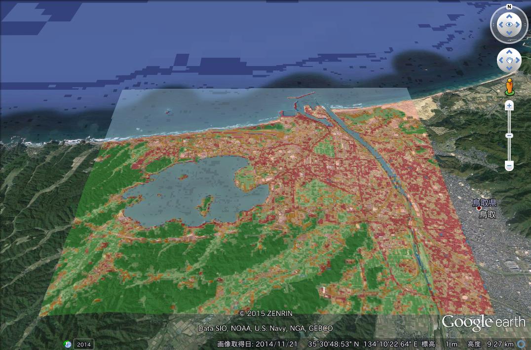
可視光の地図
|
|
rLandsat8パッケージの関数の関数が使えるようにする
|
|
放射輝度(Radiance)
|
|
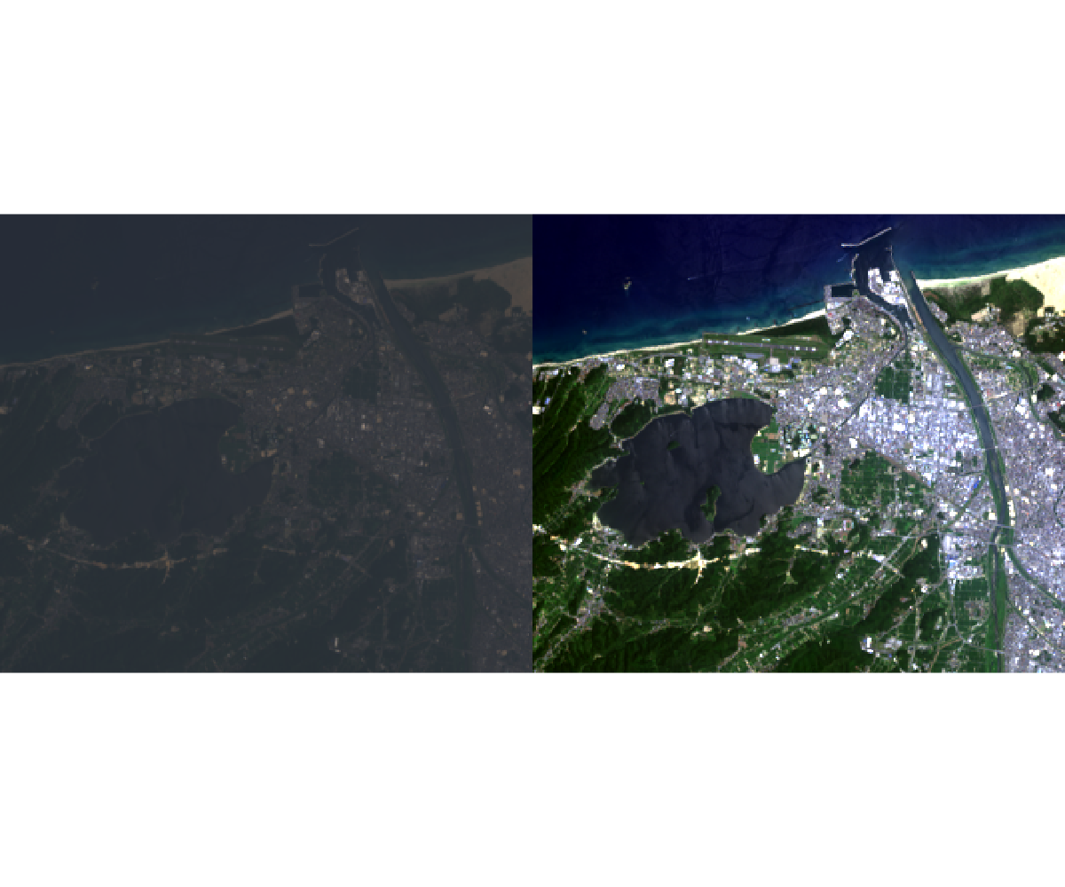
反射率(Reflectance)
太陽天頂角を考慮しない(変更前)
class : RasterLayer
dimensions : 287, 333, 95571 (nrow, ncol, ncell)
resolution : 30, 30 (x, y)
extent : 420015, 430005, 3925995, 3934605 (xmin, xmax, ymin, ymax)
coord. ref. : +proj=utm +zone=53 +datum=WGS84 +units=m +no_defs +ellps=WGS84 +towgs84=0,0,0
data source : in memory
names : blue
values : 0.09032, 0.3377 (min, max)
太陽天頂角を考慮する(変更後)
|
|
class : RasterLayer
dimensions : 287, 333, 95571 (nrow, ncol, ncell)
resolution : 30, 30 (x, y)
extent : 420015, 430005, 3925995, 3934605 (xmin, xmax, ymin, ymax)
coord. ref. : +proj=utm +zone=53 +datum=WGS84 +units=m +no_defs +ellps=WGS84 +towgs84=0,0,0
data source : in memory
names : blue
values : 0.1013435, 0.378916 (min, max)
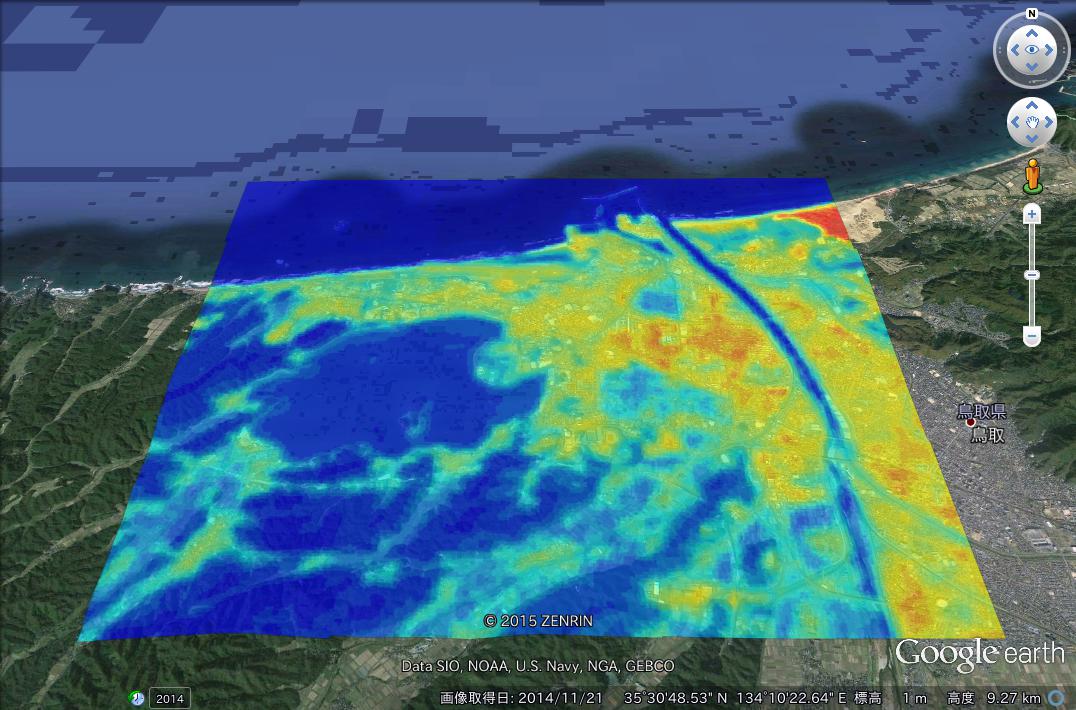
スペクトル放射輝度から温度(btemp: 絶対温度(K))
|
|
google earthに重ねると
|
|
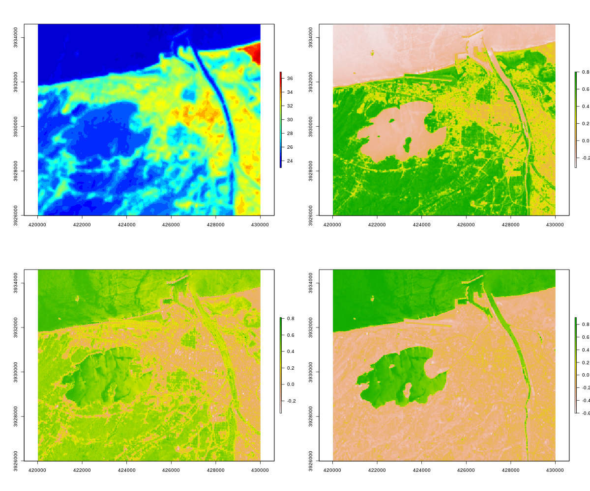
- 温度(左上) 正規化植生指数(右上)
- 地表水分指標(左下) 改良型正規化水指数(右下)
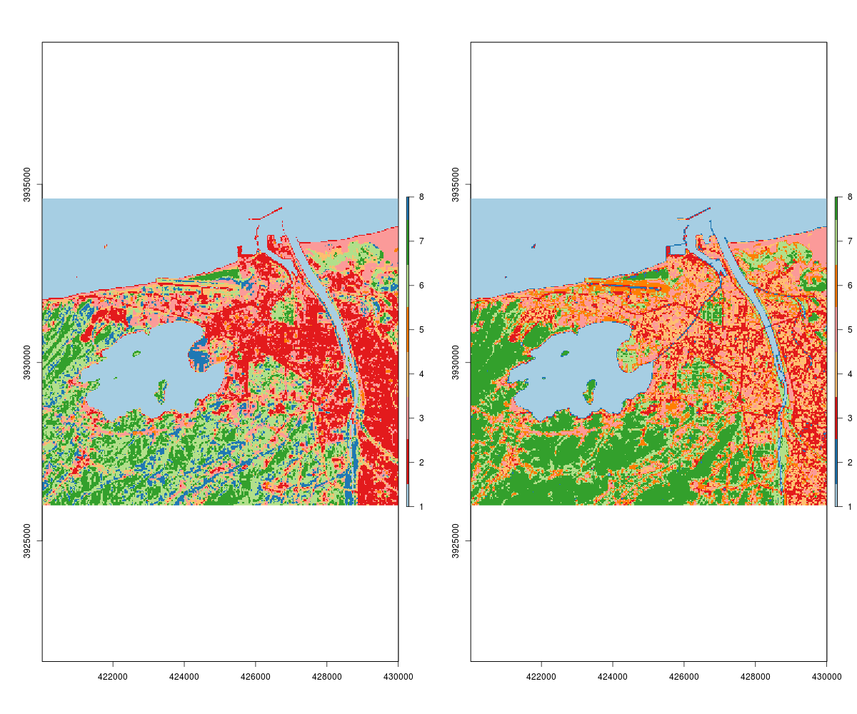
クラスタリング
aerosol 、 blue、 green、 red、 nir、 swir1、swir2 を使う
|
|
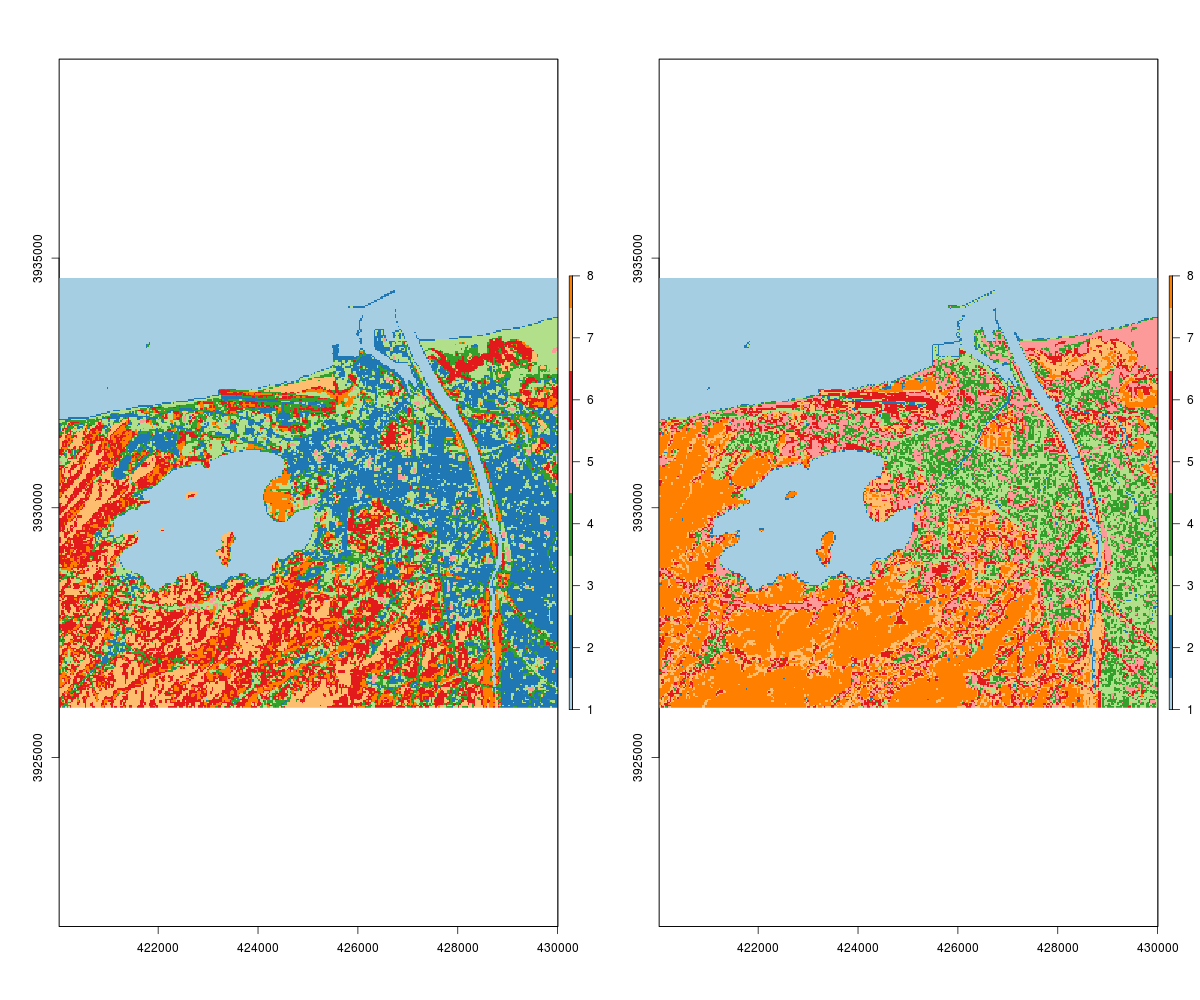
配色を変更
|
|
自己組織化マップによるクラスタリング の結果をgoogle earthで扱うためにkmz(kml)形式で保存
|
|
google earthに重ねると