縦書き帯グラフ棒グラフ

縦書き帯グラフ棒グラフ

OSはzorin os

インストールされているフォントの一覧表示:端末で、fc-list

(参考)
plotで軸タイトルを縦書きにする
Rでグラフの文字をたて書きにする

read.csvとかread.tableで文字列がfactorに解釈された場合、as.vectorで変換しないと関数がうまく働かなかった。

1
2
3
4
5
6
7
8
9
tate <- function(x){
x<-as.vector(x)
for(i in 1:length(x)){
xx<-chartr("ー", "|",x[i])
xx<-unlist(strsplit(xx,""))
x[i]<-paste(xx,collapse= "\n")
}
return(x)
}

今回はフォントも指定(linux場合の指定方法)

帯グラフ(データは家計調査より)

1
2
3
4
5
6
7
8
9
10
data<-c(0.22,0.06,0.07,0.03,0.04,0.04,0.17,0.06,0.10,0.21)
names(data)<-c("食料","住居","光熱・水道","家具・家事用品","被服及び履物","保健医療","交通・通信","教育","教養娯楽","その他の消費支出")
library(RColorBrewer)
d<-as.matrix(100 * data/ sum(data))
#png("obi01.png",width=1000,height=400)
par(family="TakaoExMincho",mar=c(5,4,5,4))
barplot(d,horiz = T,col = brewer.pal(10,"Set3"))
text(cumsum(d)-d/2,1.2-0.5,tate(colnames(t(d))),cex=1.5)
title("消費支出 項目別割合")
#dev.off()

モノクロ

1
2
3
4
5
6
7
#png("obi01_2.png",width=1000,height=400)
par(family="TakaoExMincho",mar=c(5,4,5,4))
barplot(d,horiz = T, col=c("lightgray","gray","darkgray"), lwd=1:2, angle=c(135,45,45), density=c(rep(5,3),rep(10,3),rep(20,3),100))
barplot(d,horiz = T, add=TRUE, col=c("lightgray","gray","darkgray"), lwd=1:2, angle=c(135,45,135), density=c(rep(5,3),rep(10,3),rep(20,3),100))
text(cumsum(d)-d/2,1.2-0.5,tate(colnames(t(d))),cex=1.5)
title("消費支出 項目別割合")
#dev.off()

棒グラフ

データは
平成26年賃金構造基本統計調査 結果の概況
統計表
付表7 都道府県、性、主な産業別賃金及び産業計の年齢・勤続年数(3-1)

1
2
3
4
5
6
7
8
9
10
都道府県<-c("北海道","青森","岩手","宮城","秋田","山形","福島","茨城","栃木","群馬","埼玉","千葉","東京","神奈川",
"新潟","富山","石川","福井","山梨","長野","岐阜","静岡","愛知","三重","滋賀","京都","大阪","兵庫",
"奈良","和歌山","鳥取","島根","岡山","広島","山口","徳島","香川","愛媛","高知","福岡","佐賀","長崎",
"熊本","大分","宮崎","鹿児島","沖縄")
所定内給与額<-c(259.1,226.6,234.6,272.1,241.4,242.5,260.1,288.9,290.1,277.3,294.7,299.5,377.4,336.0,262.2,275.4,278.5,271.4,283.8,
276.4,275.2,292.9,312.5,290.3,292.0,301.5,321.9,289.0,294.9,266.6,251.5,250.8,271.9,283.6,264.2,260.8,269.9,261.4,
250.9,277.3,241.8,245.4,251.5,256.5,238.2,251.8,227.7)
#データフレームに変換
#(本来は変換の必要はないけれど、Rコマンダーを使うことを想定。)
x<-data.frame(都道府県,所定内給与額)

horiz=T

鳥取だけ色を変えた。

1
2
3
4
5
#png("bou01.png",width=1000,height=1000)
barplot(rev(x[,2]),names=rev(x[,1]),las=1,cex.names=0.8,horiz=T,col=c(rep("lightblue",16),"pink",rep("lightblue",30)),
main="都道府県別所定内給与額(千円)")
abline(v=seq(100,400,100),col="blue",lty=3)
#dev.off()

tate関数を使う。

1
2
3
4
5
6
7
8
9
#png("bou02.png",width=1000,height=800)
par(family="TakaoExMincho",mar=c(10,5,5,1))
b<-barplot(x[,2],names=NA,las=1,col=c(rep("lightblue",30),"pink",rep("lightblue",16)),main="平成26年賃金構造基本統計調査:都道府県別所定内給与額(千円)")
text(b[1:47,],-5,labels=tate(x[,1]),srt=0,col=c(rep("black",30),"red",rep("black",16)),xpd=TRUE,pos=1)
abline(h=seq(100,400,100),col="gray",lty=3)
#全国計 299.6
abline(h=299.6,col="red",lty=2)
text(0.5,299.6,"全国計 299.6",col="red",pos=3)
#dev.off()

2 項目(都道府県別、性別)のデータ

1
2
3
4
5
6
7
8
9
10
11
12
13
14
15
16
17
18
19
20
21
22
23
24
25
#man<-scan("clipboard")
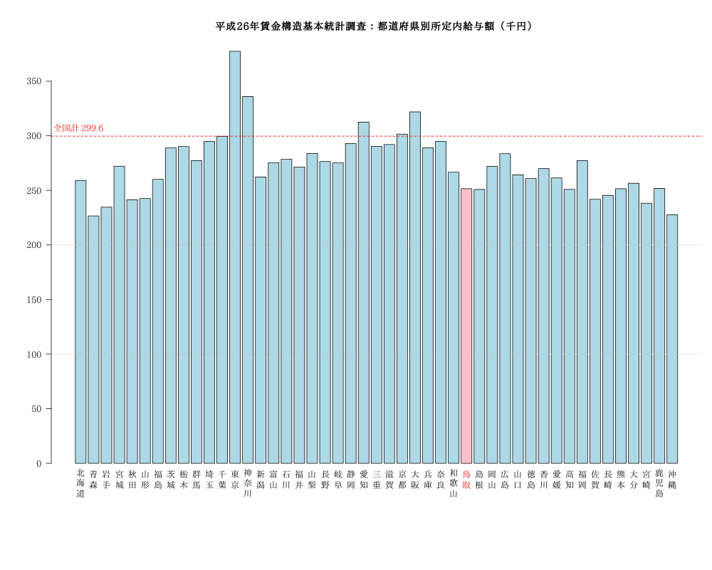
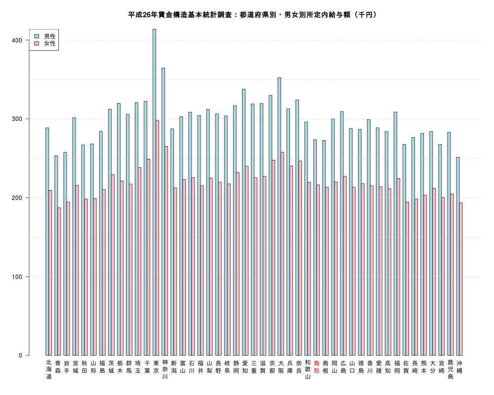
man<-c(288.6,253.3,257.7,301.6,266.9,268.2,284.3,312.3,319.6,305.8,320.6,322.3,413.8,364.4,287.4,302.7,
308.5,304.2,312.0,306.2,303.7,316.8,337.8,318.9,319.5,330.0,352.2,312.7,323.9,296.1,273.6,272.7,300.0,
309.3,287.9,286.7,299.1,288.7,283.9,308.6,267.5,276.4,281.6,283.8,267.6,283.0,251.4)
#woman<-scan("clipboard")
woman<-c(209.4,187.2,194.6,215.8,198.4,198.8,210.5,229.2,221.3,217.3,238.3,248.9,298.0,265.2,212.5,223.2,
225.5,215.4,225.2,219.8,217.6,231.9,240.0,225.4,227.2,247.6,257.8,240.3,246.6,219.7,216.2,213.4,220.2,
227.2,213.5,217.9,215.4,214.0,211.5,224.3,194.6,198.5,203.0,211.9,200.4,204.8,193.6)
kyuyo<-data.frame(man,woman)
#都道府県名をrownamesに入れる。変数に入れるより転置する際扱いやすい。
rownames(kyuyo)<-c("北海道","青森","岩手","宮城","秋田","山形","福島","茨城","栃木","群馬","埼玉","千葉","東京","神奈川",
"新潟","富山","石川","福井","山梨","長野","岐阜","静岡","愛知","三重","滋賀","京都","大阪","兵庫",
"奈良","和歌山","鳥取","島根","岡山","広島","山口","徳島","香川","愛媛","高知","福岡","佐賀","長崎",
"熊本","大分","宮崎","鹿児島","沖縄")
head(kyuyo);tail(kyuyo)
#データを転置してグラフにする。names=rep("",47)と指定
png("bou03.png",width=1000,height=800)
b<-barplot(t(kyuyo), col = c("lightblue", "pink"), beside = TRUE,las=1,names=rep("",47))
#今回は戻り値bは2行47列の行列。各列1,2行の平均をx座標とする。
text((b[2,1:47]+b[1,1:47])/2,-5,labels=tate(colnames(t(kyuyo))),srt=0,xpd=TRUE,pos=1,col=c(rep("black",30),"red",rep("black",16)))
abline(h=seq(100,400,50),col="gray",lty=3)
#legend("topleft", legend = rownames(t(kyuyo)),bg = "white", fill = c("lightblue", "pink"))
legend("topleft", legend =c("男性","女性"),bg = "white", fill = c("lightblue", "pink"))
title("平成26年賃金構造基本統計調査:都道府県別・男女別所定内給与額(千円)")
#dev.off()