forecast、tseries、timsac
(とても勉強になったサイト)
logics of blue
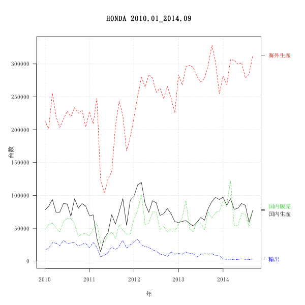
データはホンダHPから入手。
手入力した部分もあるので間違いがあるかもしれません。
|
|
honda.datを作業ディレクトリへ保存
読み込んでグラフ化
|
|
使用するパッケージ
|
|
|
|
Phillips-Perron Unit Root Test
data: data
Dickey-Fuller = -5.0908, Truncation lag parameter = 3, p-value = 0.01
|
|
Augmented Dickey-Fuller Test
data: data
Dickey-Fuller = -5.1195, Lag order = 0, p-value = 0.01
alternative hypothesis: stationary
|
|
Augmented Dickey-Fuller Test
data: data
Dickey-Fuller = -2.8843, Lag order = 3, p-value = 0.2179
alternative hypothesis: stationary
|
|
出力は省略
|
|
|
|
Box-Pierce test
data: fit$residuals
X-squared = 0.2984, df = 1, p-value = 0.5849
残差が独立である仮説が採択される
|
|
Jarque Bera Test
data: fit$residuals
X-squared = 4.7357, df = 2, p-value = 0.09368
有意水準が5%でも帰無仮説は保留され (p > 0.05)、データは正規性をもつと判断できる。
|
|
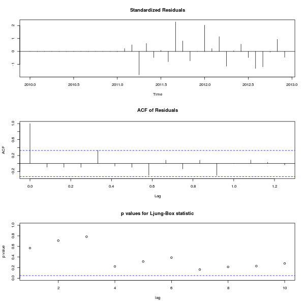
- 1番上が残差のプロット。2番目が残差の自己相関。これはなるべく小さい方がよい。
- 3番目が残差が「ホワイトノイズ」になっているかの検定プロット。
- 丸い点が上の方にあって、青い線を下回らないようであれば、ホワイトノイズと見なすこ とができる。
|
|