gdata、xts、quantmod、lattice、tseries、vars、MSBVAR、urcaパッケージ
原油価格推移では日次データはwtiとbrentのみ。
dubaiデータは
東京商品取引所のサイトにありました。
ヒストリカルデータ -> ドバイ原油ドル換算価格(月間)
これの限月:一月先を使います。
データをダウンロード -> データをつなげる(2015/1まで) -> 一月先のデータだけを抽出。
抽出にはgawkを使いました。
BEGIN { FS=”,” ; OFS=”,” }
($1~/^….01..$/) && ($5~/^….02$/){print $1,$5,$6,$7,$8,$9}
($1~/^….02..$/) && ($5~/^….03$/){print $1,$5,$6,$7,$8,$9}
($1~/^….03..$/) && ($5~/^….04$/){print $1,$5,$6,$7,$8,$9}
($1~/^….04..$/) && ($5~/^….05$/){print $1,$5,$6,$7,$8,$9}
($1~/^….05..$/) && ($5~/^….06$/){print $1,$5,$6,$7,$8,$9}
($1~/^….06..$/) && ($5~/^….07$/){print $1,$5,$6,$7,$8,$9}
($1~/^….07..$/) && ($5~/^….08$/){print $1,$5,$6,$7,$8,$9}
($1~/^….08..$/) && ($5~/^….09$/){print $1,$5,$6,$7,$8,$9}
($1~/^….09..$/) && ($5~/^….10$/){print $1,$5,$6,$7,$8,$9}
($1~/^….10..$/) && ($5~/^….11$/){print $1,$5,$6,$7,$8,$9}
($1~/^….11..$/) && ($5~/^….12$/){print $1,$5,$6,$7,$8,$9}
($1~/^….12..$/) && ($5~/^….01$/){print $1,$5,$6,$7,$8,$9}
2015年2月分はグラフ化するときにダウンロード。一月先のデータだけを抽出。つなぐ。(現在2015/2/7)
1 2 3 4 5 6 7 8 9 10 11 12 13 14 15 16 17 18 19
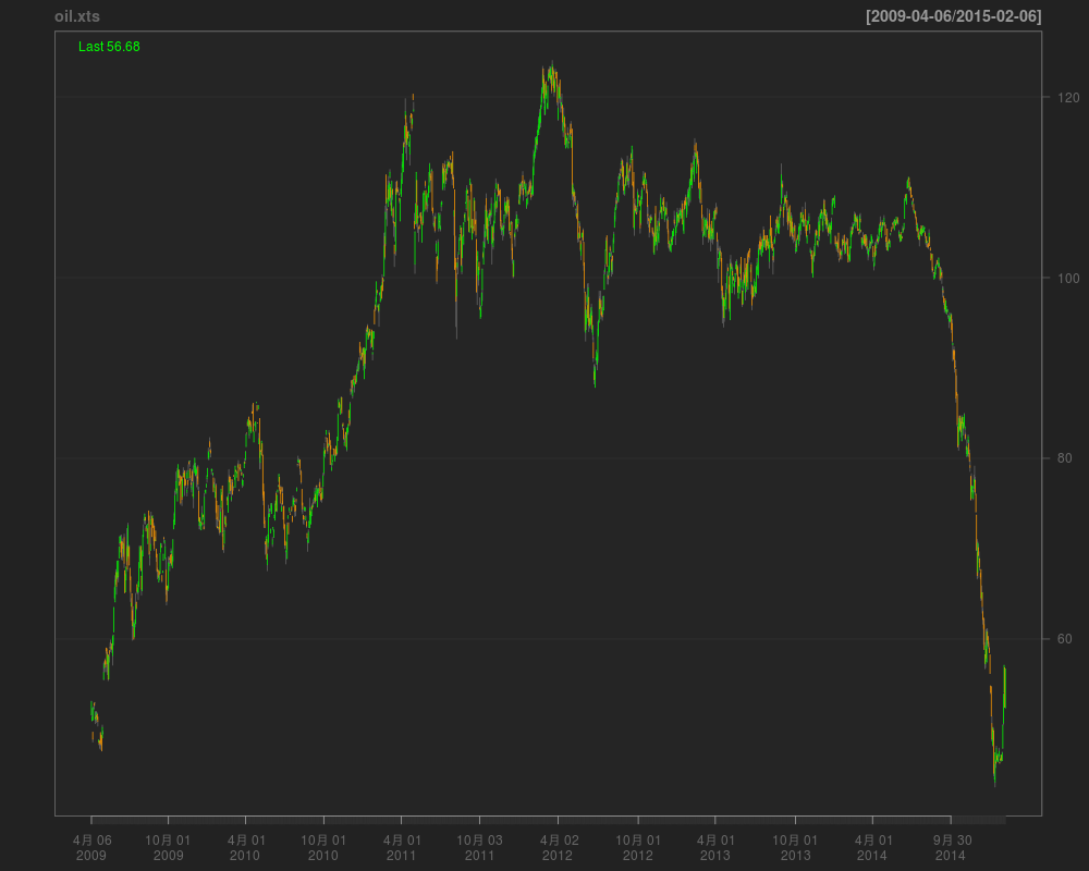
| library(xts) library(gdata) library(quantmod) library(lattice) Dubaioil200904_201501 <- read.csv("Dubaioil200904_201501_1.txt", header=TRUE) oil201502<-read.csv("http://www.tocom.or.jp/data/dollar_monthly/Pricelist_1233_201502.csv", header=F) #2月分のデータはV4==201503のデータだけ抽出 #ここではV4(限月)が営業日付の1ヶ月先のデータをグラフ化している oil02 <- subset(oil201502, subset=V5=="201503", select=c(V1,V5,V6,V7,V8,V9)) names(oil02)<-c("date", "Maturity","open","high","low","close") oil<-rbind(Dubaioil200904_201501,oil02) #月末には新しく作成したデータフレームを保存しておくと、 #新たに読み込むデータが1月分ですむ。 x <- strptime(oil[,1], format = "%Y%m%d", tz="") oil.xts<-as.xts(zoo(oil[,c(3:6)]),as.POSIXct(x)) head(oil.xts);tail(oil.xts) #png("dubai01.png",width=1000,height=800) chartSeries(oil.xts) #dev.off()
|
1 2 3 4 5 6 7
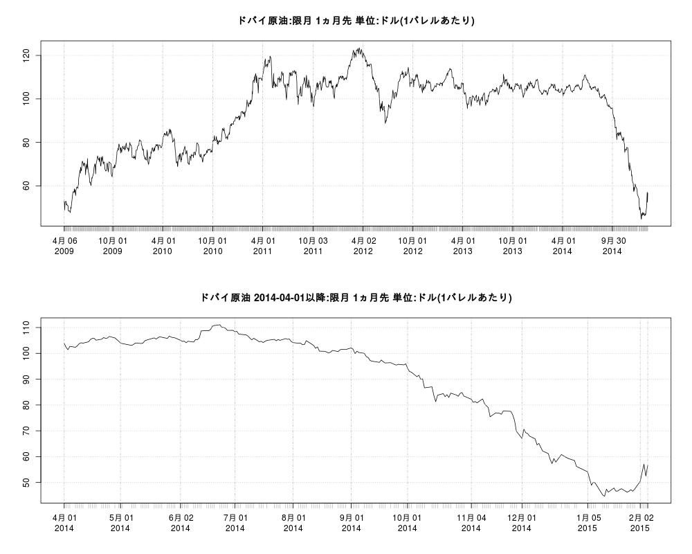
| #png("dubai02.png",width=1000,height=800) par(mfrow=c(2,1)) #終値のみのグラフ plot(oil.xts[,"close"],main="ドバイ原油:限月 1ヵ月先 単位:ドル(1バレルあたり)") #2014-04-01以降のデータ plot(oil.xts["2014-04-01::","close"],main="ドバイ原油 2014-04-01以降:限月 1ヵ月先 単位:ドル(1バレルあたり)") #dev.off()
|
1 2 3 4 5 6 7 8 9 10 11 12 13 14 15 16 17 18 19 20 21
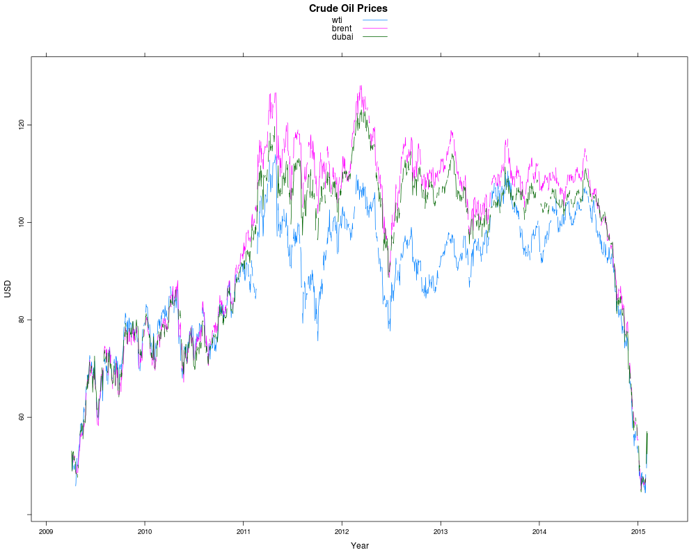
| dubai<-data.frame(as.Date(index(oil.xts)),coredata(oil.xts[,"close"])) names(dubai)<-c("date","dubai") dubai$date<-strptime(dubai$date,format ="%Y-%m-%d") d1<-read.xls("http://www.eia.gov/dnav/pet/hist_xls/RCLC1d.xls",sheet=2,skip=3,header=F) d2<-read.xls("http://www.eia.gov/dnav/pet/hist_xls/RBRTEd.xls",sheet=2,skip=3,header=F) wti<-d1;brent<-d2 names(wti)<-c("date","wti") names(brent)<-c("date","brent") Sys.setlocale("LC_TIME", "C") wti$date<-strptime(wti$date,format ="%b %d%Y") brent$date<-strptime(brent$date,format ="%b %d%Y") oil0 <- merge(wti,brent, all=T) oil <- merge(oil0,dubai,by="date", all=T) oil.xts <- as.xts(zoo(oil[,-1]), as.POSIXct(oil[,1])) xyplot(oil.xts['2009-04-05::'], superpose=TRUE, xlab="Year", ylab="USD",main="Crude Oil Prices")
|
1 2 3 4
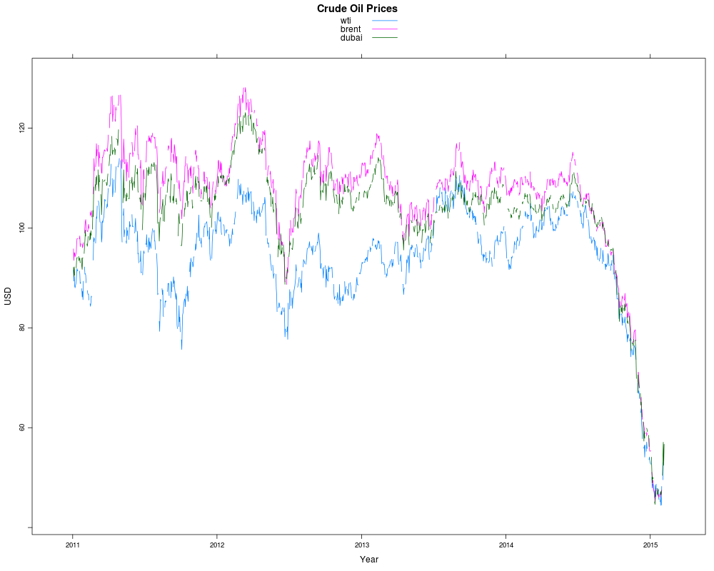
| xyplot(oil.xts['2011-01-01::'], superpose=TRUE, xlab="Year", ylab="USD",main="Crude Oil Prices")
|
以下はRのコードを見つけたからやってみただけです。
(計量経済学とか)勉強したことすらありません。
Toda-Yamamoto implementation in ‘R’に書いてあるやり方。
1 2 3 4 5 6 7 8 9 10 11 12 13 14 15 16 17 18 19 20 21 22 23 24 25 26 27 28 29 30 31 32 33 34 35 36 37 38 39 40 41 42
| #グランジャー因果 library(fUnitRoots) library(urca) library(vars) library(aod) library(zoo) library(tseries) # [1] (wti と dubaiについて)欠損値のあるデータを削除。 x<-na.omit(data.frame(coredata(oil.xts['2011-01-01::',c("wti","dubai")]))) #個々の原系列に対して単位根検定を実施 adf.test(x$wti);adf.test(x$dubai) adf.test(diff(x$wti,lag=1));adf.test(diff(x$dubai,lag=1)) VARselect(x[,c("wti","dubai")],lag=10,type="both") #VAR-Model, lag=1 V.1<-VAR(x[,c("wti","dubai")],p=1,type="both") #plot(V.1) serial.test(V.1) #VAR Model, lag=2 V.2<-VAR(x[,c("wti","dubai")],p=2,type="both") #plot(V.2) serial.test(V.2) #有意でないlag=2について、もっと調べる。 #for (i in 1:10){ #Vs<-serial.test(VAR(x[,c("wti","dubai")],i,type="both")) #print(i);print(Vs) #} #Stability analysis 1/roots(V.2)[[1]] # ">1" 1/roots(V.2)[[2]] # ">1" #Alternative stability analyis plot(stability(V.2)) #lag=2を採用する #VAR-Model, lag=2+1=3 V.3<-VAR(x[,c("wti","dubai")],p=3,type="both") V.3$varresult summary(V.3) #Wald-test (H0: dubai does not Granger-cause wti) wald.test(b=coef(V.3$varresult[["wti"]]), Sigma=vcov(V.3$varresult[["wti"]]), Terms=c(2,4)) # 5%水準で有意である。H0を棄却する。 (X2 = 15.6, df = 2, P(> X2) = 0.00042) #Wald.test (H0: wti does not Granger-cause dubai) wald.test(b=coef(V.3$varresult[["dubai"]]), Sigma=vcov(V.3$varresult[["dubai"]]), Terms= c(1,3)) # 5%水準で有意でない。H0を棄却できない。 (X2 = 0.45, df = 2, P(> X2) = 0.8)
|
- dubai -> wti にgranger因果あり
1 2 3 4 5 6 7 8 9 10 11 12 13 14 15 16 17 18 19 20 21 22 23 24 25 26 27 28 29 30 31 32 33 34 35 36 37
| # [2] (wti と brentについて)欠損値のあるデータを削除。 x<-na.omit(data.frame(coredata(oil.xts['2011-01-01::',c("wti","brent")]))) #ccf(x[,1],x[,2]) #個々の原系列に対して単位根検定を実施 adf.test(x$wti);adf.test(x$brent) adf.test(diff(x$wti,lag=1));adf.test(diff(x$brent,lag=1)) VARselect(x[,c("wti","brent")],lag=10,type="both") #VAR Model, lag=2 V.2<-VAR(x[,c("wti","brent")],p=2,type="both") #plot(V.2) serial.test(V.2) #VAR-Model, lag=4 V.4<-VAR(x[,c("wti","brent")],p=4,type="both") #plot(V.4) serial.test(V.4) #lag=2,4とも有意(有意水準:5%) #比較的ましなlag=4について調べる。 #for (i in 1:10){ #Vs<-serial.test(VAR(x[,c("wti","brent")],i,type="both")) #print(i);print(Vs) #} #Stability analysis 1/roots(V.4)[[1]] # ">1" 1/roots(V.4)[[2]] # ">1" #Alternative stability analyis plot(stability(V.4)) #lag=4を採用する #VAR-Model, lag=4+1=5 V.5<-VAR(x[,c("wti","brent")],p=5,type="both") V.5$varresult summary(V.5) #Wald-test (H0: brent does not Granger-cause wti) wald.test(b=coef(V.5$varresult[["wti"]]), Sigma=vcov(V.5$varresult[["wti"]]), Terms=c(2,4,6,8)) # 5%水準で有意でない。H0を棄却できない。 (X2 = 3.1, df = 4, P(> X2) = 0.54) #Wald.test (H0: wti does not Granger-cause brent) wald.test(b=coef(V.5$varresult[["brent"]]), Sigma=vcov(V.5$varresult[["brent"]]), Terms= c(1,3,5,7)) # 5%水準で有意である。H0を棄却する。 (X2 = 64.6, df = 4, P(> X2) = 3.1e-13)
|
- wti -> brent にgranger因果あり
1 2 3 4 5 6 7 8 9 10 11 12 13 14 15 16 17 18 19 20 21 22 23 24 25 26 27 28 29 30 31 32 33
| # [3] (dubai と brentについて)欠損値のあるデータを削除。 x<-na.omit(data.frame(coredata(oil.xts['2011-01-01::',c("dubai","brent")]))) #ccf(x[,1],x[,2]) #個々の原系列に対して単位根検定を実施 adf.test(x$dubai);adf.test(x$brent) adf.test(diff(x$dubai,lag=1));adf.test(diff(x$brent,lag=1)) VARselect(x[,c("dubai","brent")],lag=10,type="both") #VAR Model, lag=3 V.3<-VAR(x[,c("dubai","brent")],p=3,type="both") #plot(V.3) serial.test(V.3) #lag=3は有意でない。一応、調べる # #for (i in 1:10){ #Vs<-serial.test(VAR(x[,c("dubai","brent")],i,type="both")) #print(i);print(Vs) #} #Stability analysis 1/roots(V.3)[[1]] # ">1" 1/roots(V.3)[[2]] # ">1" #Alternative stability analyis plot(stability(V.3)) #lag=3を採用する #VAR-Model, lag=3+1=4 V.4<-VAR(x[,c("dubai","brent")],p=4,type="both") V.4$varresult summary(V.4) #Wald-test (H0: brent does not Granger-cause dubai) wald.test(b=coef(V.4$varresult[["dubai"]]), Sigma=vcov(V.4$varresult[["dubai"]]), Terms=c(2,4,6)) # 5%水準で有意でない。H0を棄却できない。 (X2 = 1.3, df = 3, P(> X2) = 0.73) #Wald.test (H0: dubai does not Granger-cause brent) wald.test(b=coef(V.4$varresult[["brent"]]), Sigma=vcov(V.4$varresult[["brent"]]), Terms= c(1,3,5)) # 5%水準で有意である。H0を棄却する。 (X2 = 194.4, df = 3, P(> X2) = 0.0)
|
debai -> brent にgranger因果あり
(まとめ) グランジャー因果があるのは
dubai -> wti
wti -> brent
dubai -> brent
ググると見かける手順。
1 2 3 4 5 6 7 8 9 10 11 12 13 14 15 16 17 18 19 20 21 22 23 24 25 26
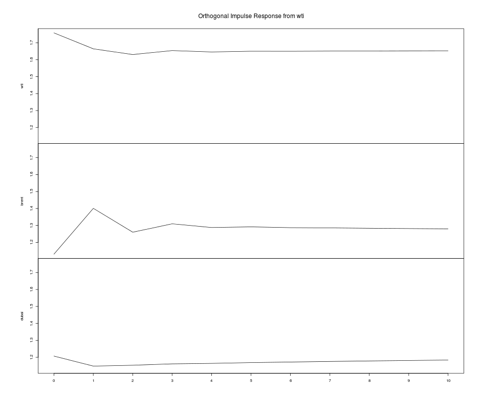
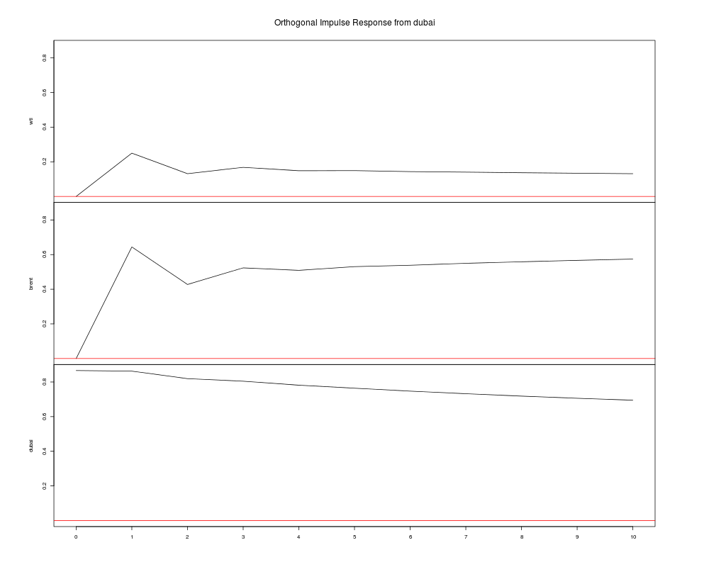
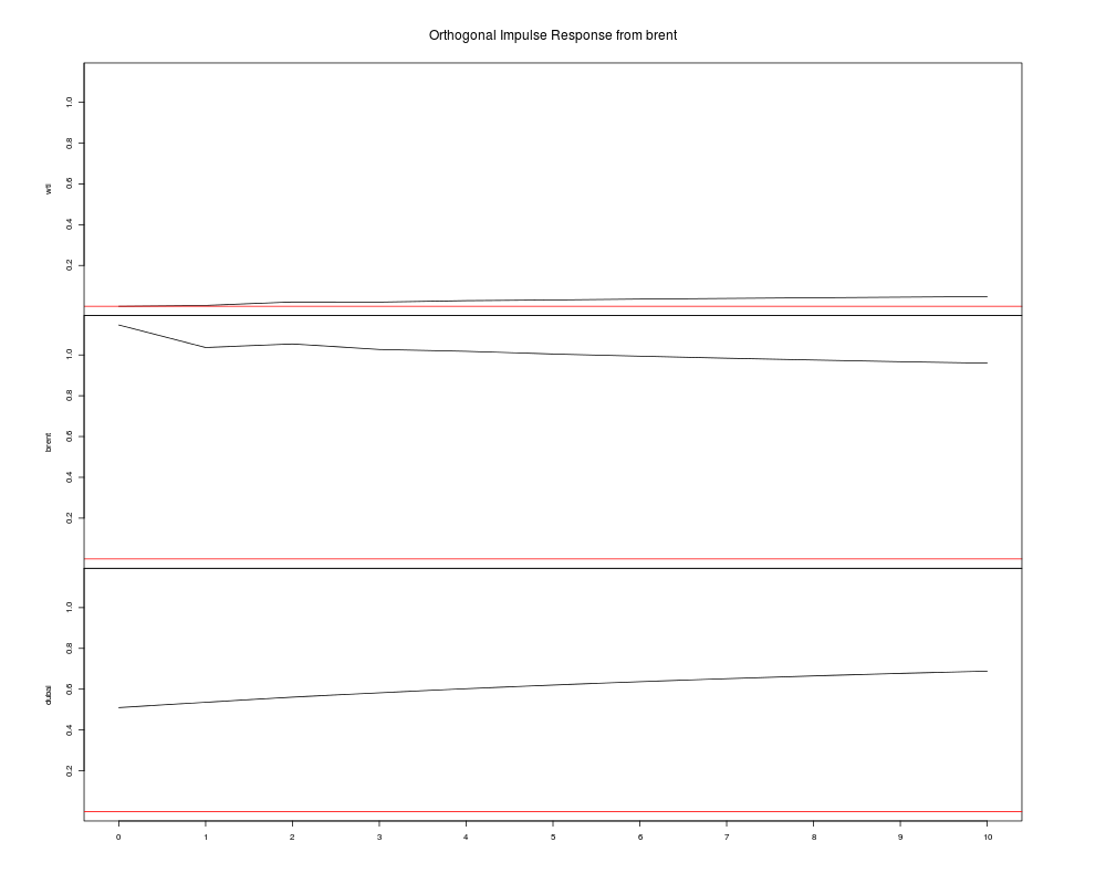
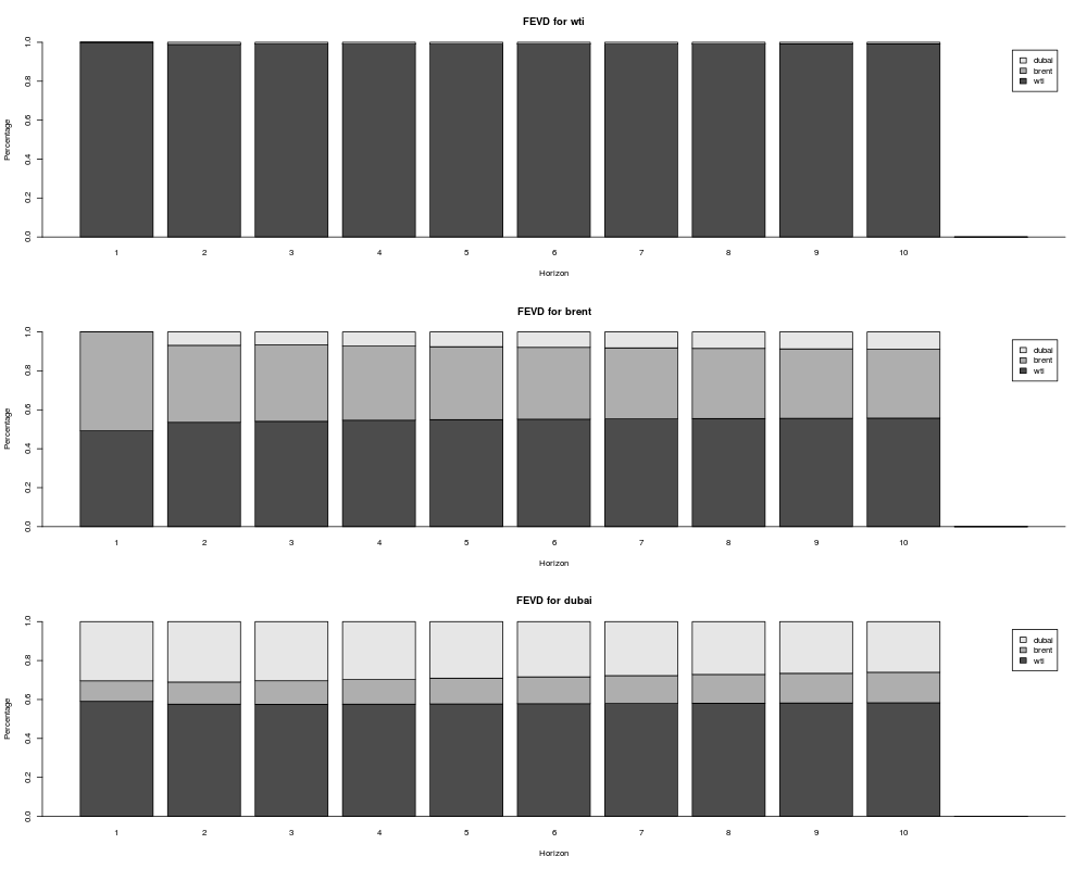
| x<-na.omit(data.frame(coredata(oil.xts['2011-01-01::']))) po.test(x) # 有意でない。が、 oil.vecm<-ca.jo(x,ecdet="none",type="eigen",K=2,spec="longrun") urca::summary(oil.vecm) #共和分ランクはr=1 #plot(oil.vecm) #plotres(oil.vecm) #oil.vec.rls=cajorls(oil.vecm,r=1) #oil.vec.rls$rlm #lttest(oil.vecm, r=2) oil.vec2var<-vec2var(oil.vecm,r=1) print(oil.vec2var) #arch.test(oil.vec2var) #normality.test(oil.vec2var) #serial.test(oil.vec2var) plot(vars::irf(oil.vec2var,boot=F, impulse ="wti")) plot(vars::irf(oil.vec2var,boot=F, impulse ="dubai")) plot(vars::irf(oil.vec2var,boot=F, impulse ="brent")) ## plot(fevd(oil.vec2var)) #class(oil.vec2var) #methods(class = "vec2var") #oil.predict<-predict(oil.vec2var,n.head=50) #plot(oil.predict) #fanchart(oil.predict)
|
インパルス応答推定
予測誤差分散分解
共和分がなかったとしたら、
1 2 3 4
| x.d<-data.frame(wti=diff(x$wti,lag=1),brent=diff(x$brent,lag=1),dubai=diff(x$dubai,lag=1)) VARselect(x.d) library(MSBVAR) granger.test(x.d, p=4)
|
F-statistic p-value
brent -> wti 1.1433213 3.348290e-01
dubai -> wti 4.7223787 9.057081e-04
wti -> brent 7.3341979 8.463202e-06
dubai -> brent 47.1208944 0.000000e+00
wti -> dubai 0.3881335 8.172167e-01
brent -> dubai 2.0902467 8.031484e-02
偏granger(Partial Granger causality)
1 2 3 4 5 6 7 8 9 10 11 12 13 14 15 16 17 18 19
| #FIAR library(Matrix) library(np) #library(lavaan) library(devtools) #FIAR:FIARパッケージはcranにはもうないが、githubに関数があったので読み込んで使う。 source_url('https://raw.githubusercontent.com/cran/FIAR/master/R/partGranger.R') #Partial Granger causality #使い方はよく分からない for (i in 1:3){ for (j in 1:3){ if (i!=j){ x.d_c<-data.frame(x.d[,c(i,j)],x.d[-c(i,j)]) pG<-partGranger(x.d_c,nx=1,ny=1,order=4) pGr<-paste(colnames(x.d_c[1]),"->",colnames(x.d_c[2]),round(pG$orig,6),round(pG$prob,6)) print(pGr,quote=F) } } }
|
wti -> brent 0.010944 0.077814
wti -> dubai 0.006317 0.302918
brent -> wti 0.043463 1e-06
brent -> dubai 0.031341 7.7e-05
dubai -> wti 0.029121 0.00017
dubai -> brent 0.175752 0
Granger causality とは違って、
- wti -> brent の因果なし。
- brent -> wti , brent -> dubai の因果あり。
Granger causality については、素人がやってみただけのことです。 信用はされないようにお願いします。