WDI,data.table,reshape2,countrycode パッケージ
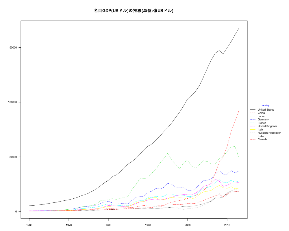
G7(フランス、アメリカ、日本、イタリア、カナダ、イギリス、ドイツ)のGNPの推移
世界銀行のデータを使ってグラフにする。
iso2cは “FR”,”US”,”JP”,”IT”,”CA”,”DE”,”GB”ってなかなか覚えられない。
検索してみると、国コード一覧CSV ISO 3166-1発見。
(準備)
これとcountrycodeパッケージのcountrycode_dataとをマージした。
csvファイルに書き出して、日本語の国名を短く(アメリカ合衆国をアメリカのように)した。
countrycodeJP.csvというファイル名で作業フォルダに保存。
手順
|
|
検索にはdata.table パッケージを使うと便利
data.frameのsubsetより、記述が簡単で検索が速い。
|
|
|
|
表は省略
ある地域(ここではEastern Asia)のGDPの成長率
|
|

|
|
| year | Macao.SAR..China | Mongolia | China | Korea..Rep. | Hong.Kong.SAR..China | Japan | Korea..Dem..Rep. |
|---|---|---|---|---|---|---|---|
| 1960 | NA | NA | NA | NA | NA | NA | NA |
| 1961 | NA | NA | -27.30 | 4.94 | NA | 12.04 | NA |
| 1962 | NA | NA | -5.60 | 2.46 | NA | 8.91 | NA |
| 1963 | NA | NA | 10.20 | 9.53 | NA | 8.47 | NA |
| 1964 | NA | NA | 18.30 | 7.56 | NA | 11.68 | NA |
| 1965 | NA | NA | 17.00 | 5.19 | NA | 5.82 | NA |
| 1966 | NA | NA | 10.70 | 12.70 | 1.79 | 10.64 | NA |
| 1967 | NA | NA | -5.70 | 6.10 | 1.60 | 11.08 | NA |
| 1968 | NA | NA | -4.10 | 11.70 | 3.40 | 12.88 | NA |
| 1969 | NA | NA | 16.90 | 14.10 | 11.34 | 12.48 | NA |
| 1970 | NA | NA | 19.40 | 12.87 | 9.21 | -1.02 | NA |
| 1971 | NA | NA | 7.00 | 10.44 | 7.29 | 4.70 | NA |
| 1972 | NA | NA | 3.80 | 6.51 | 10.61 | 8.41 | NA |
| 1973 | NA | NA | 7.90 | 14.79 | 12.28 | 8.03 | NA |
| 1974 | NA | NA | 2.30 | 9.38 | 2.42 | -1.23 | NA |
| 1975 | NA | NA | 8.70 | 7.34 | 0.49 | 3.09 | NA |
| 1976 | NA | NA | -1.60 | 13.46 | 16.16 | 3.97 | NA |
| 1977 | NA | NA | 7.60 | 11.82 | 11.73 | 4.39 | NA |
| 1978 | NA | NA | 11.67 | 10.30 | 8.26 | 5.27 | NA |
| 1979 | NA | NA | 7.57 | 8.39 | 11.56 | 5.48 | NA |
| 1980 | NA | NA | 7.84 | -1.89 | 10.11 | 2.82 | NA |
| 1981 | NA | NA | 5.24 | 7.40 | 9.26 | 4.18 | NA |
| 1982 | NA | 8.34 | 9.06 | 8.29 | 2.95 | 3.38 | NA |
| 1983 | 10.00 | 5.83 | 10.85 | 12.18 | 5.98 | 3.06 | NA |
| 1984 | 8.50 | 5.93 | 15.18 | 9.86 | 9.97 | 4.46 | NA |
| 1985 | 0.70 | 5.71 | 13.47 | 7.47 | 0.76 | 6.33 | NA |
| 1986 | 6.70 | 9.37 | 8.85 | 12.24 | 11.06 | 2.83 | NA |
| 1987 | 14.30 | 3.46 | 11.58 | 12.27 | 13.40 | 4.11 | NA |
| 1988 | 7.80 | 5.11 | 11.28 | 11.66 | 8.51 | 7.15 | NA |
| 1989 | 5.00 | 4.18 | 4.06 | 6.75 | 2.28 | 5.37 | NA |
| 1990 | 8.00 | -3.18 | 3.84 | 9.30 | 3.83 | 5.57 | NA |
| 1991 | 3.70 | -8.69 | 9.18 | 9.71 | 5.70 | 3.32 | NA |
| 1992 | 13.30 | -9.26 | 14.24 | 5.77 | 6.23 | 0.82 | NA |
| 1993 | 5.20 | -3.17 | 13.96 | 6.33 | 6.20 | 0.17 | NA |
| 1994 | 4.30 | 2.13 | 13.08 | 8.77 | 6.04 | 0.87 | NA |
| 1995 | 3.30 | 6.38 | 10.92 | 8.93 | 2.37 | 1.94 | NA |
| 1996 | -0.40 | 2.24 | 10.01 | 7.19 | 4.26 | 2.61 | NA |
| 1997 | -0.30 | 3.90 | 9.30 | 5.77 | 5.10 | 1.60 | NA |
| 1998 | -4.60 | 3.34 | 7.83 | -5.71 | -5.88 | -2.00 | NA |
| 1999 | -2.40 | 3.07 | 7.62 | 10.73 | 2.51 | -0.20 | NA |
| 2000 | 5.70 | 1.15 | 8.43 | 8.83 | 7.66 | 2.26 | NA |
| 2001 | 2.90 | 2.95 | 8.30 | 4.53 | 0.56 | 0.36 | NA |
| 2002 | 8.90 | 4.73 | 9.08 | 7.43 | 1.66 | 0.29 | NA |
| 2003 | 12.59 | 7.00 | 10.03 | 2.93 | 3.06 | 1.69 | NA |
| 2004 | 26.88 | 10.63 | 10.09 | 4.90 | 8.70 | 2.36 | NA |
| 2005 | 8.56 | 7.25 | 11.31 | 3.92 | 7.39 | 1.30 | NA |
| 2006 | 14.42 | 8.56 | 12.68 | 5.18 | 7.03 | 1.69 | NA |
| 2007 | 14.33 | 10.25 | 14.16 | 5.46 | 6.46 | 2.19 | NA |
| 2008 | 3.39 | 8.90 | 9.63 | 2.83 | 2.13 | -1.04 | NA |
| 2009 | 1.71 | -1.27 | 9.21 | 0.71 | -2.46 | -5.53 | NA |
| 2010 | 27.50 | 6.37 | 10.45 | 6.50 | 6.77 | 4.65 | NA |
| 2011 | 21.29 | 17.51 | 9.30 | 3.68 | 4.79 | -0.45 | NA |
| 2012 | 9.14 | 12.40 | 7.65 | 2.29 | 1.55 | 1.75 | NA |
| 2013 | 11.89 | 11.74 | 7.67 | 2.97 | 2.93 | 1.61 | NA |
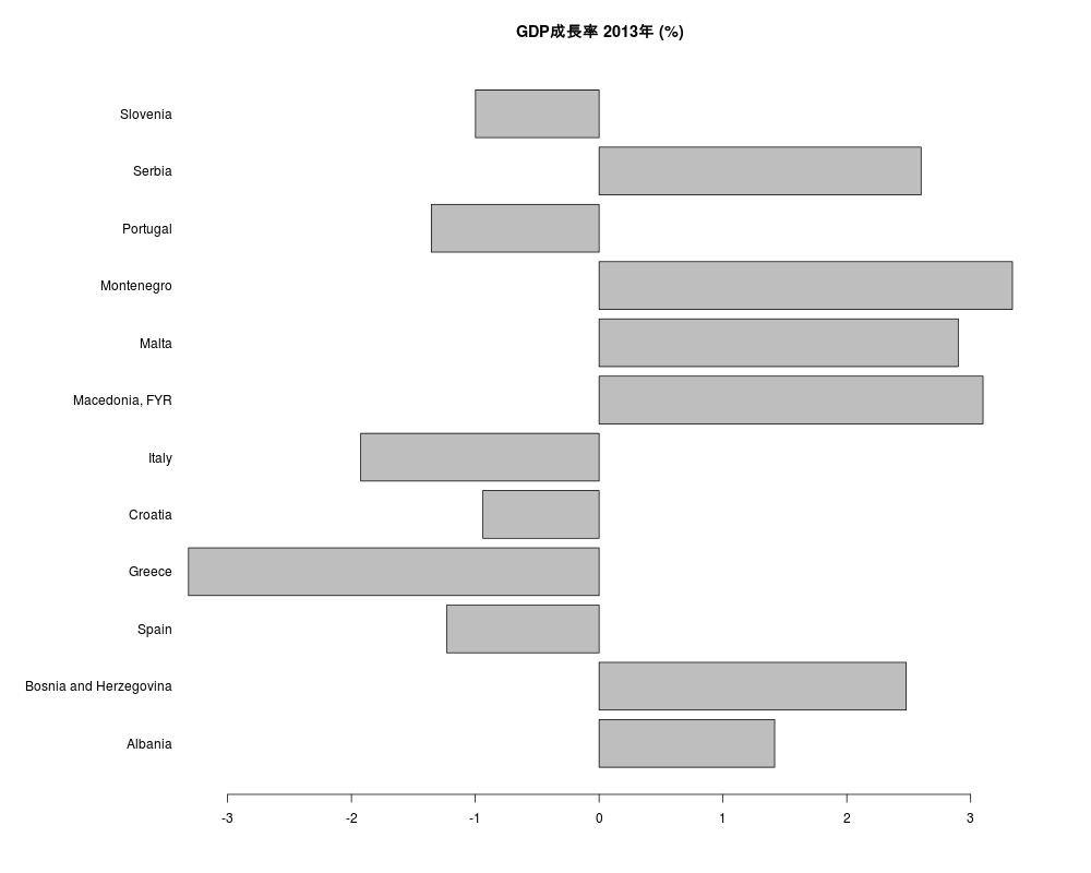
Southern EuropeのGDPの成長率(2013年)
|
|