放送大学「心理統計法(‘17)」第10章 その 3
授業ではrstanパッケージを使ってますが、MCMCpackパッケージを使ってみます。初学者ですので間違いが多々あると思います。
(Rスクリプトはここ)
早稲田大学文学部文学研究科 豊田研究室
(参考)
ベイジアンMCMCによる統計モデル
Using the ggmcmc package
Bayesian Inference With Stan ~番外編~
Exercise 2: Bayesian A/B testing using MCMC Metropolis-Hastings
政治学方法論 I
|
|
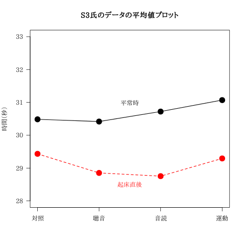
推測例3(2水準の主効果の分析)
|
|
|
|
| 平常時 対照 | 平常時 聴音 | 平常時 音読 | 平常時 運動 | 起床直後 対照 | 起床直後 聴音 | 起床直後 音読 | 起床直後 運動 | |
|---|---|---|---|---|---|---|---|---|
| 平均 | 30.48 | 30.42 | 30.72 | 31.07 | 29.43 | 28.85 | 28.75 | 29.29 |
| 標準偏差 | 2.40 | 1.99 | 1.90 | 1.90 | 2.98 | 1.91 | 1.59 | 3.60 |
|
|
|
|
| EAP | post.sd | 2.5% | 5% | 50% | 95% | 97.5% | |
|---|---|---|---|---|---|---|---|
| mu | 29.88 | 0.29 | 29.32 | 29.41 | 29.88 | 30.35 | 30.44 |
| muA1 | 0.08 | 0.50 | -0.89 | -0.73 | 0.08 | 0.90 | 1.05 |
| muA2 | -0.24 | 0.50 | -1.23 | -1.07 | -0.24 | 0.57 | 0.73 |
| muA3 | -0.14 | 0.50 | -1.11 | -0.95 | -0.14 | 0.67 | 0.84 |
| muA4 | 0.30 | 0.49 | -0.67 | -0.51 | 0.30 | 1.11 | 1.27 |
| muB1 | 0.79 | 0.29 | 0.23 | 0.33 | 0.79 | 1.26 | 1.36 |
| muB2 | -0.79 | 0.29 | -1.36 | -1.26 | -0.79 | -0.33 | -0.23 |
| muAB11 | -0.27 | 0.49 | -1.25 | -1.08 | -0.27 | 0.54 | 0.70 |
| muAB12 | 0.27 | 0.49 | -0.70 | -0.54 | 0.27 | 1.08 | 1.25 |
| muAB21 | -0.01 | 0.49 | -0.98 | -0.83 | -0.02 | 0.80 | 0.96 |
| muAB22 | 0.01 | 0.49 | -0.96 | -0.80 | 0.02 | 0.83 | 0.98 |
| muAB31 | 0.19 | 0.50 | -0.79 | -0.63 | 0.19 | 1.01 | 1.17 |
| muAB32 | -0.19 | 0.50 | -1.17 | -1.01 | -0.19 | 0.63 | 0.79 |
| muAB41 | 0.09 | 0.50 | -0.88 | -0.73 | 0.09 | 0.91 | 1.07 |
| muAB42 | -0.09 | 0.50 | -1.07 | -0.91 | -0.09 | 0.73 | 0.88 |
| sigmaE | 2.54 | 0.22 | 2.16 | 2.21 | 2.53 | 2.93 | 3.02 |
水準とセルの効果の評価
P.147 (9.12)式
水準・交互作用の効果が0より大きい(小さい)確率
|
|
| muA1 | muA2 | muA3 | muA4 | muB1 | muB2 | muAB11 | muAB12 | muAB21 | muAB22 | muAB31 | muAB32 | muAB41 | muAB42 | |
|---|---|---|---|---|---|---|---|---|---|---|---|---|---|---|
| 0 < | 0.566 | 0.31 | 0.39 | 0.728 | 0.997 | 0.003 | 0.29 | 0.71 | 0.487 | 0.513 | 0.654 | 0.346 | 0.573 | 0.427 |
| =< 0 | 0.434 | 0.69 | 0.61 | 0.272 | 0.003 | 0.997 | 0.71 | 0.29 | 0.513 | 0.487 | 0.346 | 0.654 | 0.427 | 0.573 |
要因の効果の評価
|
|
| EAP | post.sd | 2.5% | 5% | 50% | 95% | 97.5% | |
|---|---|---|---|---|---|---|---|
| sigmaA | 0.496 | 0.211 | 0.142 | 0.183 | 0.477 | 0.874 | 0.960 |
| sigmaB | 0.795 | 0.285 | 0.235 | 0.325 | 0.794 | 1.265 | 1.359 |
| sigmaAB | 0.482 | 0.207 | 0.140 | 0.178 | 0.462 | 0.853 | 0.939 |
| sigmaE | 2.544 | 0.218 | 2.162 | 2.215 | 2.528 | 2.926 | 3.017 |
| etaA2 | 0.037 | 0.028 | 0.003 | 0.005 | 0.030 | 0.092 | 0.108 |
| etaB2 | 0.090 | 0.054 | 0.007 | 0.014 | 0.084 | 0.190 | 0.212 |
| etaAB2 | 0.035 | 0.027 | 0.003 | 0.004 | 0.028 | 0.087 | 0.103 |
| etat2 | 0.162 | 0.061 | 0.056 | 0.069 | 0.158 | 0.269 | 0.291 |
| deltaA | 0.195 | 0.082 | 0.057 | 0.073 | 0.189 | 0.340 | 0.372 |
| deltaB | 0.315 | 0.115 | 0.091 | 0.126 | 0.315 | 0.505 | 0.540 |
| deltaAB | 0.190 | 0.080 | 0.056 | 0.071 | 0.183 | 0.331 | 0.362 |