震源地と原子力発電所(世界その0)

ggplot2 , maps , mapdata , geosphere , RCurl パッケージ

(過去の記事)
アメリカ地質調査所 ( 平成28年(2016年)熊本地震 )
震源地と原子力発電所03

1
2
3
4
5
6
7
8
9
10
11
12
13
14
15
16
17
18
19
20
21
22
23
24
25
26
27
28
29
30
31
32
33
34
35
36
37
38
39
40
41
42
43
44
45
46
47
48
49
50
51
52
53
54
55
56
57
58
59
60
61
62
63
64
65
66
67
68
69
70
71
72
73
74
75
76
77
78
79
80
81
82
83
84
85
86
87
88
89
90
91
92
93
94
95
96
97
98
99
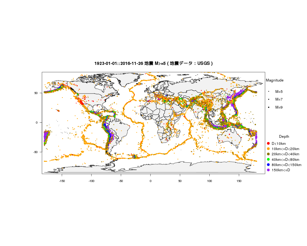
library(RCurl)
library(mapdata)
library(xts)
#
lon=c(-180,180)
lat=c(-90,90)
#
minmagnitude<-5
#
#一括処理(USGS:地震データダウンロード。保存。)
#震源データをダウンロードする年
start<-1923 ; end<-2016
library(RCurl)
for (i in start:end){
year<-as.character(i)
#format=csvとする
url<-paste0("http://earthquake.usgs.gov/fdsnws/event/1/query?format=csv&starttime=",as.numeric(year),"-01-01&endtime=",as.numeric(year)+1,
"-01-01&minmagnitude=",minmagnitude,"&minlatitude=",lat[1],"&maxlatitude=",lat[2],"&minlongitude=",lon[1],"&maxlongitude=",lon[2],"&eventtype=earthquake")
doc <- getURL(url)
filename<-paste0("USGS",year,"_",lon[1],"_",lon[2],"_",lat[1],"_",lat[2],".csv")
out <- file(filename, "w") # 書き込みモードで開く
writeLines(doc,out,sep = "\n")
close(out)
}
#
#eq
eq<-read.table(text="",col.names=c("time","latitude","longitude","depth","mag"))
for (i in start:end){
year<-as.character(i)
filename<-paste0("USGS",year,"_",lon[1],"_",lon[2],"_",lat[1],"_",lat[2],".csv")
tmp<-read.csv(filename)
#eqdata <- subset(tmp, select=c(time,latitude,longitude,depth,mag,nst,gap,dmin,rms))
tmp <- subset(tmp, select=c(time,latitude,longitude,depth,mag))
eq<-rbind(eq,tmp)
}
#
#save(eq,file="usgs5_1923_20161126.RData")
#
#USGS:地震データ
eqdata <- subset(eq, select=c(time,longitude,latitude,depth,mag))
#head(eqdata)
eqdata$time<-gsub("T"," ",substring(eqdata[,1],1,19))
eq.xts<-as.xts(read.zoo(eqdata))
ymd<-"1923-01-01::2016-11-26"
eqdata<-data.frame(coredata(eq.xts[ymd]))
#
#震源の深さ
# depth<10km
eqdata1<-subset(eqdata,depth<10)
eqdata1$depth_rank<-" 10km 未満"
eqdata1$col<-"red"
# 10<=depth<20
eqdata2<-subset(eqdata,depth>=10 & depth<20)
eqdata2$depth_rank<-" 10km以上20km未満"
eqdata2$col<-"orange"
# 20<=depth<40
eqdata3<-subset(eqdata,depth>=20 & depth<40)
eqdata3$depth_rank<-" 20km以上40km未満"
eqdata3$col<-"gold4"
# 40<=depth<80
eqdata4<-subset(eqdata,depth>=40 & depth<80)
eqdata4$depth_rank<-" 40km以上80km未満"
eqdata4$col<-"green"
# 80<=depth<150
eqdata5<-subset(eqdata,depth>=80 & depth<150)
eqdata5$depth_rank<-" 80km以上150km未満"
eqdata5$col<-"blue"
# 150<=depth
eqdata6<-subset(eqdata,depth>=150)
eqdata6$depth_rank<-"150km以上"
eqdata6$col<-"purple"
#
eq<-rbind(eqdata1,eqdata2,eqdata3,eqdata4,eqdata5,eqdata6)
#並べ替え:マグニチュードの昇順
sortlist <- order(eq$mag)
subeq<- eq[sortlist,]
##
#
par(family = "TakaoExMincho")
#png("world1923_20161126.png",width=1000,height=800)
map('world',fill=T,col="gray95",mar = c(5,4,4,15))
#map('worldHires',fill=T,col="gray95",mar = c(5,4,4,15))
points(subeq$longitude,subeq$latitude,cex=subeq$mag/15,col=adjustcolor(subeq$col,1),pch=19)
par(xpd=T)
#
cexsize=c(5,7,9)/15
legend(par("usr")[2]*1.001,par("usr")[3]*0.05+par("usr")[4]*0.95,title="Magnitude",
legend = c("M=5","M=7","M=9"),
col=1,pch=19,pt.cex=cexsize,
cex =1, x.intersp = 2, y.intersp =1.8,bty = "n")
#
legend(par("usr")[2],par("usr")[3]*0.6+par("usr")[4]*0.4,title="Depth",
legend = c("D<10km","10km<=D<20km","20km<=D<40km","40km<=D<80km","80km<=D<150km","150km<=D"),
cex=1,pch=19,col=c("red","orange","gold4","green","blue","purple"),
pt.cex =1.5,bg ="gray90", x.intersp = 1, y.intersp =1.2,bty = "n")
par(xpd=F)
title(paste0(ymd," 地震 M>=5 ( 地震データ:USGS )"))
map.axes(cex.axis=0.8,las=1)
#dev.off()
世界の原発の近くで発生した地震をプロット

(注意)日本の場合、USGSのデータは気象庁のデータより位置の精度が低いようです。

1
2
3
4
5
6
7
8
9
10
11
12
13
14
15
16
17
18
19
20
21
22
23
24
25
26
27
28
29
30
31
32
33
34
35
36
37
38
39
40
41
42
43
44
45
46
47
48
49
50
51
52
53
54
55
56
57
58
59
60
61
62
63
64
65
66
library("ggplot2")
library("maps")
#library("mapdata")
library("geosphere")
#library(gridExtra)
load("in_service.dat")
sortlist <- order(in_service$Country)
( nuclear <- in_service[sortlist,] )
#
world = map_data("worldHires")
#
#200km
d=200000
#
for (i in 1:nrow(nuclear)) {
lon1<-destPointRhumb(c(nuclear$longitude[i],nuclear$latitude[i]), 270, d, r = 6378137)[1]
lon2<-destPointRhumb(c(nuclear$longitude[i],nuclear$latitude[i]), 90, d, r = 6378137)[1]
Lon.range = c(lon1,lon2)
#
lon1<-destPointRhumb(c(nuclear$longitude[i],nuclear$latitude[i]), 180, d, r = 6378137)[2]
lon2<-destPointRhumb(c(nuclear$longitude[i],nuclear$latitude[i]), 0, d, r = 6378137)[2]
Lat.range = c(lon1,lon2)
#Lon.range = c(nuclear$longitude[i]-0.5, nuclear$longitude[i]+0.5)
#Lat.range = c(nuclear$latitude[i]-0.5, nuclear$latitude[i]+0.5)
##
p<-ggplot() +
borders("world",fill="gray75", size = 0.3) +
theme_bw() +
coord_map(xlim=Lon.range ,ylim=Lat.range) +
labs(y="",x="")
#マグニチュード5以上
eq1=subeq[ subeq$mag>=5,]
p<-p + geom_point(data=eq1, aes(x=longitude, y=latitude,fill=depth_rank,size=mag),alpha=0.8,shape=21,color="gray20")+
#プロットする色を指定したい場合
scale_fill_manual(values=c("red","orange","gold4","green","blue","purple"),
breaks = c(" 10km 未満"," 10km以上20km未満"," 20km以上40km未満"," 40km以上80km未満"," 80km以上150km未満","150km以上"))+
#プロットする大きさの範囲を指定したい場合
scale_size(breaks=c(5,6,7,8,9),range = c(3,10)) +
# 凡例のタイトルの指定
labs(size="Magnitude",fill="Depth",title=paste(nuclear$Country[i],"震源分布(マグニチュード5以上)1923 ~ 2016-11-26[データ:USGS]")) +
#凡例の順番を入れ替える
guides(size = guide_legend(order = 1), fill = guide_legend(order = 2)) +
theme(text=element_text(size=12, family="TakaoExMincho"))
p<- p + geom_point(data=nuclear,aes(x=longitude, y=latitude),shape=24,size =5, fill=rgb(0,0,0,0.8),color="black")
p<- p + geom_text(data=nuclear[i,],aes(x=longitude, y=latitude, label = station),vjust = 0, nudge_y = 0.06)
#30km円
circle30=as.data.frame(destPoint(c(nuclear$longitude[i],nuclear$latitude[i]), b=1:365, d=30000))
p<-p + geom_polygon(data=circle30, aes(x=lon,y=lat), color="black",fill="red",alpha=0.12)
p<-p + geom_text(aes(x=nuclear$longitude[i],y=max(circle30$lat)),label="30km", nudge_y = 0.04)
#50km円
circle50=as.data.frame(destPoint(c(nuclear$longitude[i],nuclear$latitude[i]), b=1:365, d=50000))
p<-p + geom_polygon(data=circle50, aes(x=lon,y=lat), color="black",fill="blue",alpha=0.12)
p<-p + geom_text(aes(x=nuclear$longitude[i],y=max(circle50$lat)),label="50km", nudge_y = 0.04)
#100km円
circle100=as.data.frame(destPoint(c(nuclear$longitude[i],nuclear$latitude[i]), b=1:365, d=100000))
p<-p + geom_polygon(data=circle100, aes(x=lon,y=lat), color="black",fill="green",alpha=0.12)
p<-p + geom_text(aes(x=nuclear$longitude[i],y=max(circle100$lat)),label="100km", nudge_y = 0.04)
#150km円
circle150=as.data.frame(destPoint(c(nuclear$longitude[i],nuclear$latitude[i]), b=1:365, d=150000))
p<-p + geom_polygon(data=circle150, aes(x=lon,y=lat), color="black",fill="yellow",alpha=0.12)
p<-p + geom_text(aes(x=nuclear$longitude[i],y=max(circle150$lat)),label="150km", nudge_y = 0.04)
#
png(paste0("nuclearworld",i,".png"),width=800,height=600)
print(p)
dev.off()
}

地図は次からの記事