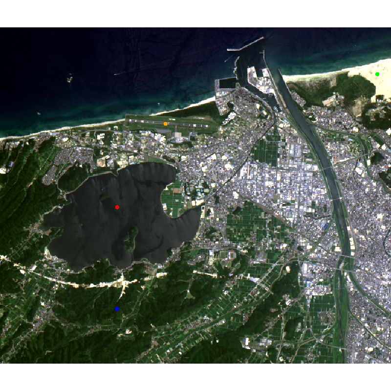
library(raster) library(colorRamps) library(RColorBrewer) library(rLandsat8) ToTOAReflectance <- function(landsat8, band) { bandnames <- c("aerosol", "blue", "green", "red", "nir", "swir1", "swir2", "panchromatic", "cirrus", "tirs1", "tirs2") idx <- seq_along(bandnames)[sapply(bandnames, function(x) band %in% x)] ml <- as.numeric(landsat8$metadata[[paste0("reflectance_mult_band_", idx)]]) al <- as.numeric(landsat8$metadata[[paste0("reflectance_add_band_", idx)]]) TOAref <- (landsat8$band[[band]] * ml + al)/sin(as.numeric(landsat8$metadata$sun_elevation) * pi /180) return(TOAref) } ToMNDWI <- function(landsat8) { green <- ToTOAReflectance(landsat8, "green") swir1 <- ToTOAReflectance(landsat8, "swir1") mndwi <- (green - swir1) / (green + swir1) return(mndwi) } read.meta<- function(product){ meta.file <- paste0(product, "/", product, "_MTL.txt") textLines <- readLines(meta.file) met <- read.table(text=textLines[grep("=", textLines)],header = FALSE, sep = "=", strip.white = TRUE, stringsAsFactors = FALSE,row.names = NULL, col.names = c("name", "value")) met <- met[!met$name == "GROUP", ] met <- met[!met$name == "END_GROUP", ] rownames(met) <- tolower(met[, "name"]) met[, "name"] <- NULL met <- as.list(as.data.frame(t(met), stringsAsFactors = FALSE)) return(met) } panSharpen <- function(img, pan, r, g, b) { stopifnot(inherits(img, "Raster") & inherits(pan, "Raster")) layernames <- names(img)[c(r,g,b)] ordr <- match(layernames, names(img)) layernames <- layernames[order(ordr)] msi <- resample(img[[layernames]], pan, method = "ngb") mult <- pan / sum(msi) panimg <- msi * mult names(panimg) <- paste0(layernames, "_pan") panimg } setwd("/media/user/MUSIC") product <- "LC81110352015214LGN00" Crop <- c(420000,430000,3926000,3934600) meta<-read.meta(product) date<-meta$date_acquired fname<-paste0(fname0,substr(date,1,4),substr(date,6,7),substr(date,9,10)) OLI<-stack(c(aerosol=paste0(product,"/",product, "_B1.TIF"),blue=paste0(product,"/",product, "_B2.TIF"), green=paste0(product,"/",product, "_B3.TIF"),red=paste0(product,"/",product, "_B4.TIF"), nir=paste0(product,"/",product, "_B5.TIF"),swir1=paste0(product,"/",product, "_B6.TIF"), swir2=paste0(product,"/",product, "_B7.TIF"),cirrus=paste0(product,"/",product, "_B9.TIF"))) PAN <-stack(paste0(product,"/",product, "_B8.TIF")) names(PAN)<-"panchromatic" TIRS<-stack(c(tirs1=paste0(product,"/",product, "_B10.TIF"),tirs2=paste0(product,"/",product, "_B11.TIF"))) subOLI <- crop(OLI,Crop) subPAN <- crop(PAN,Crop) subTIRS <- crop(TIRS,Crop) bands=c(unstack(subOLI)[1:7],unstack(subPAN),unstack(subOLI)[8],unstack(subTIRS)) l<-list(metadata = meta, band = bands) names(l$band)<-c("aerosol","blue", "green", "red","nir","swir1","swir2","panchromatic","cirrus","tirs1","tirs2") RGBpan <- panSharpen(stack(l$band[2:4]),l$band$panchromatic, r = 3, g = 2, b = 1) pos1<-c(423000,3930000) pos2<-c(423000,3927400) pos3<-c(429650,3933400) pos4<-c(424240,3932130) plotRGB(RGBpan,r = 3, g = 2, b = 1,stretch="lin") points(pos1[1],pos1[2],col="red",pch=16,cex=1.5) points(pos2[1],pos2[2],col="blue",pch=16,cex=1.5) points(pos3[1],pos3[2],col="green",pch=16,cex=1.5) points(pos4[1],pos4[2],col="orange",pch=16,cex=1.5) l_ref<-stack(ToTOAReflectance(landsat8=l, band="aerosol"), ToTOAReflectance(landsat8=l, band="blue"), ToTOAReflectance(landsat8=l, band="green"), ToTOAReflectance(landsat8=l, band="red"), ToTOAReflectance(landsat8=l, band="nir"), ToTOAReflectance(landsat8=l, band="swir1"), ToTOAReflectance(landsat8=l, band="swir2")) l_ref_cor<-stack(radiocorr(l,band="aerosol",method = "DOS1"), radiocorr(l,band="blue",method = "DOS1"), radiocorr(l,band="green",method = "DOS1"), radiocorr(l,band="red",method = "DOS1"), radiocorr(l,band="nir",method = "DOS1"), radiocorr(l,band="swir1",method = "DOS1"), radiocorr(l,band="swir2",method = "DOS1")) l_ref_dos2<-stack(radiocorr(l,band="aerosol",method = "DOS2"), radiocorr(l,band="blue",method = "DOS2"), radiocorr(l,band="green",method = "DOS2"), radiocorr(l,band="red",method = "DOS2"), radiocorr(l,band="nir",method = "DOS2"), radiocorr(l,band="swir1",method = "DOS1"), radiocorr(l,band="swir2",method = "DOS1")) l_ref_dos4<-stack(radiocorr(l,band="aerosol",method = "DOS4"), radiocorr(l,band="blue",method = "DOS4"), radiocorr(l,band="green",method = "DOS4"), radiocorr(l,band="red",method = "DOS4"), radiocorr(l,band="nir",method = "DOS4"), radiocorr(l,band="swir1",method = "DOS4"), radiocorr(l,band="swir2",method = "DOS4")) p1 <- crop(l_ref,c(pos1[1],pos1[1]+1,pos1[2],pos1[2]+1)) p2 <- crop(l_ref,c(pos2[1],pos2[1]+1,pos2[2],pos2[2]+1)) p3 <- crop(l_ref,c(pos3[1],pos3[1]+1,pos3[2],pos3[2]+1)) p4 <- crop(l_ref,c(pos4[1],pos4[1]+1,pos4[2],pos4[2]+1)) p5 <- crop(l_ref_cor,c(pos1[1],pos1[1]+1,pos1[2],pos1[2]+1)) p6 <- crop(l_ref_cor,c(pos2[1],pos2[1]+1,pos2[2],pos2[2]+1)) p7 <- crop(l_ref_cor,c(pos3[1],pos3[1]+1,pos3[2],pos3[2]+1)) p8 <- crop(l_ref_cor,c(pos4[1],pos4[1]+1,pos4[2],pos4[2]+1)) p9 <- crop(l_ref_dos4,c(pos1[1],pos1[1]+1,pos1[2],pos1[2]+1)) p10 <- crop(l_ref_dos4,c(pos2[1],pos2[1]+1,pos2[2],pos2[2]+1)) p11 <- crop(l_ref_dos4,c(pos3[1],pos3[1]+1,pos3[2],pos3[2]+1)) p12 <- crop(l_ref_dos4,c(pos4[1],pos4[1]+1,pos4[2],pos4[2]+1)) p13 <- crop(l_ref_dos2,c(pos1[1],pos1[1]+1,pos1[2],pos1[2]+1)) p14 <- crop(l_ref_dos2,c(pos2[1],pos2[1]+1,pos2[2],pos2[2]+1)) p15 <- crop(l_ref_dos2,c(pos3[1],pos3[1]+1,pos3[2],pos3[2]+1)) p16 <- crop(l_ref_dos2,c(pos4[1],pos4[1]+1,pos4[2],pos4[2]+1)) par(mfrow=c(2,2)) plot(p1@data@min,type="o",pch=16,cex=1.5,lwd=2,col="red",xaxt = "n", xlab="Band",ylab="Reflectance",las=1,ylim=c(0,0.3),bty = "l") title("場所によるバンド別反射率の違い(大気補正なし)") axis(1, at=1:length(p1), labels=c("aerosol\n0.43-0.45μm","blue\n0.45-0.51μm", "green\n0.53-0.59μm", "red\n0.64-0.67μm","nir\n0.85-0.88μm","swir1\n1.57-1.65μm","swir2\n2.11-2.29μm"),tck=0.01) lines(p2@data@min,type="o",pch=16,cex=1.5,lwd=2,col="blue") lines(p3@data@min,type="o",pch=16,cex=1.5,lwd=2,col="green") lines(p4@data@min,type="o",pch=16,cex=1.5,lwd=2,col="orange") legend("topleft",legend=c("池","森林","砂浜","滑走路"),col=c("red","blue","green","orange"),pch=16,cex=1,lty=1) plot(p5@data@min,type="o",pch=16,cex=1.5,lwd=2,col="red",xaxt = "n", xlab="Band",ylab="Reflectance",las=1,ylim=c(0,0.3),bty = "l") title("場所によるバンド別反射率の違い(大気補正あり:DOS1)") axis(1, at=1:length(p5), labels=c("aerosol\n0.43-0.45μm","blue\n0.45-0.51μm", "green\n0.53-0.59μm", "red\n0.64-0.67μm","nir\n0.85-0.88μm","swir1\n1.57-1.65μm","swir2\n2.11-2.29μm"),tck=0.01) lines(p6@data@min,type="o",pch=16,cex=1.5,lwd=2,col="blue") lines(p7@data@min,type="o",pch=16,cex=1.5,lwd=2,col="green") lines(p8@data@min,type="o",pch=16,cex=1.5,lwd=2,col="orange") legend("topleft",legend=c("池","森林","砂浜","滑走路"),col=c("red","blue","green","orange"),pch=16,cex=1,lty=1) plot(p13@data@min,type="o",pch=16,cex=1.5,lwd=2,col="red",xaxt = "n", xlab="Band",ylab="Reflectance",las=1,ylim=c(0,0.3),bty = "l") title("場所によるバンド別反射率の違い(大気補正あり:DOS2)") axis(1, at=1:length(p1), labels=c("aerosol\n0.43-0.45μm","blue\n0.45-0.51μm", "green\n0.53-0.59μm", "red\n0.64-0.67μm","nir\n0.85-0.88μm","swir1\n1.57-1.65μm","swir2\n2.11-2.29μm"),tck=0.01) lines(p14@data@min,type="o",pch=16,cex=1.5,lwd=2,col="blue") lines(p15@data@min,type="o",pch=16,cex=1.5,lwd=2,col="green") lines(p16@data@min,type="o",pch=16,cex=1.5,lwd=2,col="orange") legend("topleft",legend=c("池","森林","砂浜","滑走路"),col=c("red","blue","green","orange"),pch=16,cex=1,lty=1) plot(p9@data@min,type="o",pch=16,cex=1.5,lwd=2,col="red",xaxt = "n", xlab="Band",ylab="Reflectance",las=1,ylim=c(0,0.3),bty = "l") title("場所によるバンド別反射率の違い(大気補正あり:DOS4)") axis(1, at=1:length(p9), labels=c("aerosol\n0.43-0.45μm","blue\n0.45-0.51μm", "green\n0.53-0.59μm", "red\n0.64-0.67μm","nir\n0.85-0.88μm","swir1\n1.57-1.65μm","swir2\n2.11-2.29μm"),tck=0.01) lines(p10@data@min,type="o",pch=16,cex=1.5,lwd=2,col="blue") lines(p11@data@min,type="o",pch=16,cex=1.5,lwd=2,col="green") lines(p12@data@min,type="o",pch=16,cex=1.5,lwd=2,col="orange") legend("topleft",legend=c("池","森林","砂浜","滑走路"),col=c("red","blue","green","orange"),pch=16,cex=1,lty=1) par(mfrow=c(1,1)) par(mfrow=c(2,2)) plot(p1@data@min,type="o",pch=16,cex=1.5,lwd=2,col="red",xaxt = "n", xlab="Band",ylab="Reflectance",las=1,ylim=c(0,0.3),bty = "l") axis(1, at=1:length(p1), labels=c("aerosol\n0.43-0.45μm","blue\n0.45-0.51μm", "green\n0.53-0.59μm", "red\n0.64-0.67μm","nir\n0.85-0.88μm","swir1\n1.57-1.65μm","swir2\n2.11-2.29μm"),tck=0.01) title("大気補正によるバンド別反射率の違い(池)") lines(p5@data@min,type="o",pch=16,cex=1.5,lwd=2,col="blue",lty=2) lines(p9@data@min,type="o",pch=16,cex=1.5,lwd=2,col="green",lty=3) lines(p13@data@min,type="o",pch=16,cex=1.5,lwd=2,col="orange",lty=4) legend("topleft",legend=c("大気補正なし","DOS1","DOS2","DOS4"),col=c("red","blue","orange","green"),pch=16,cex=1,lty=c(1,2,4,3)) plot(p2@data@min,type="o",pch=16,cex=1.5,lwd=2,col="red",xaxt = "n", xlab="Band",ylab="Reflectance",las=1,ylim=c(0,0.3),bty = "l") axis(1, at=1:length(p2), labels=c("aerosol\n0.43-0.45μm","blue\n0.45-0.51μm", "green\n0.53-0.59μm", "red\n0.64-0.67μm","nir\n0.85-0.88μm","swir1\n1.57-1.65μm","swir2\n2.11-2.29μm"),tck=0.01) title("大気補正によるバンド別反射率の違い(森林)") lines(p6@data@min,type="o",pch=16,cex=1.5,lwd=2,col="blue",lty=2) lines(p10@data@min,type="o",pch=16,cex=1.5,lwd=2,col="green",lty=3) lines(p14@data@min,type="o",pch=16,cex=1.5,lwd=2,col="orange",lty=4) legend("topleft",legend=c("大気補正なし","DOS1","DOS2","DOS4"),col=c("red","blue","orange","green"),pch=16,cex=1,lty=c(1,2,4,3)) plot(p3@data@min,type="o",pch=16,cex=1.5,lwd=2,col="red",xaxt = "n", xlab="Band",ylab="Reflectance",las=1,ylim=c(0,0.3),bty = "l") axis(1, at=1:length(p3), labels=c("aerosol\n0.43-0.45μm","blue\n0.45-0.51μm", "green\n0.53-0.59μm", "red\n0.64-0.67μm","nir\n0.85-0.88μm","swir1\n1.57-1.65μm","swir2\n2.11-2.29μm"),tck=0.01) title("大気補正によるバンド別反射率の違い(砂浜)") lines(p7@data@min,type="o",pch=16,cex=1.5,lwd=2,col="blue",lty=2) lines(p11@data@min,type="o",pch=16,cex=1.5,lwd=2,col="green",lty=3) lines(p15@data@min,type="o",pch=16,cex=1.5,lwd=2,col="orange",lty=4) legend("topleft",legend=c("大気補正なし","DOS1","DOS2","DOS4"),col=c("red","blue","orange","green"),pch=16,cex=1,lty=c(1,2,4,3)) plot(p4@data@min,type="o",pch=16,cex=1.5,lwd=2,col="red",xaxt = "n", xlab="Band",ylab="Reflectance",las=1,ylim=c(0,0.3),bty = "l") axis(1, at=1:length(p4), labels=c("aerosol\n0.43-0.45μm","blue\n0.45-0.51μm", "green\n0.53-0.59μm", "red\n0.64-0.67μm","nir\n0.85-0.88μm","swir1\n1.57-1.65μm","swir2\n2.11-2.29μm"),tck=0.01) title("大気補正によるバンド別反射率の違い(滑走路)") lines(p8@data@min,type="o",pch=16,cex=1.5,lwd=2,col="blue",lty=2) lines(p12@data@min,type="o",pch=16,cex=1.5,lwd=2,col="green",lty=3) lines(p16@data@min,type="o",pch=16,cex=1.5,lwd=2,col="orange",lty=4) legend("topleft",legend=c("大気補正なし","DOS1","DOS2","DOS4"),col=c("red","blue","orange","green"),pch=16,cex=1,lty=c(1,2,4,3)) par(mfrow=c(1,1))
|