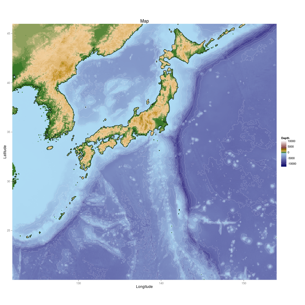
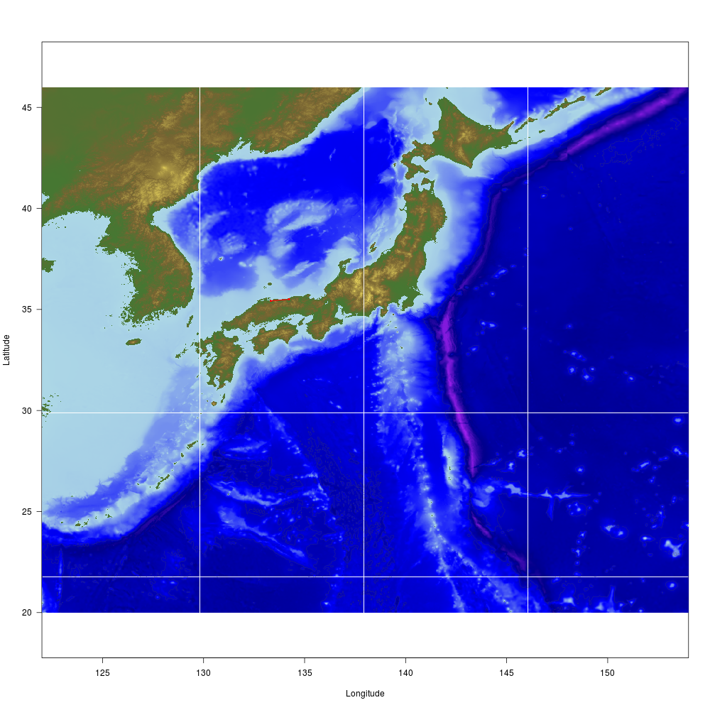
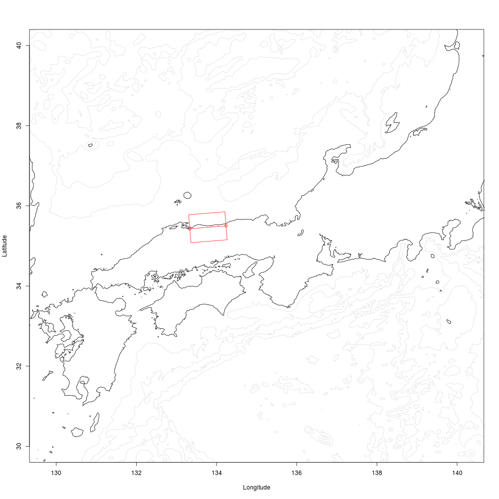
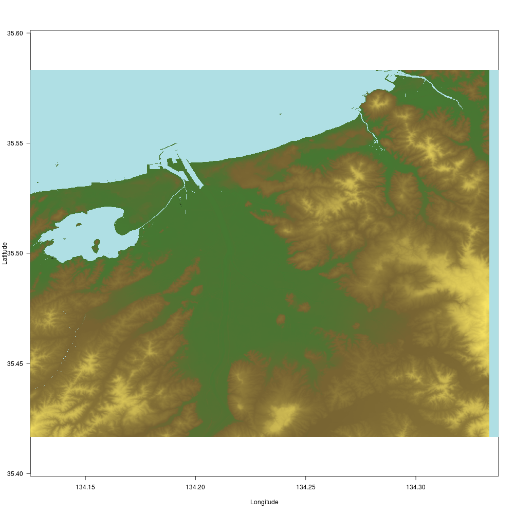
海底地形と地形データ

marmap ,ggplot2 , lattice パッケージ

(参考)Kitahashi’s Web Site

最後の地図以外は「NOAAのデータ」を使用して作成しました。

(注)
linuxにmarmapパッケージをインストールするには、ncdf パッケージのインストールが必要。
ncdf パッケージをインストールするには、
「before installing ncdf in R intall in your linux libnetcdf-dev and netcdf-bin」です。

library(marmap) ; library(ggplot2)
Lon.range = c(122, 154)
Lat.range = c(20, 46)
#ダウンロードしたデータを保存する場合は keep=T とする。
dat <- getNOAA.bathy(Lon.range[1],Lon.range[2],Lat.range[1],Lat.range[2],res=5)
# Plot bathy object using custom ggplot2 functions
#png("japan05.png",width=1000,height=1000)
autoplot(dat, geom=c("r", "c"), colour="white", size=0.1) + 
scale_fill_etopo()+ 
labs(x="Longitude",y="Latitude",fill="Depth") +
ggtitle("Map")
#dev.off()

• GMT（The Generic Mapping Tools）で作成した地図には劣りますが、こんな短いコードで「データのダウンロードから地図の作成まで」をやってくれます。

ggplot2::autoplotを使わないで作図。

library(marmap) # ; library(mapdata)
Lon.range = c(122, 154)
Lat.range = c(20, 46)
dat<-getNOAA.bathy(Lon.range[1],Lon.range[2],Lat.range[1],Lat.range[2],res=5,keep=TRUE)
#summary(dat)
oce <- colorRampPalette(c("purple","darkblue","blue","lightblue"))
land1 <- colorRampPalette(c("#467832","#786432"))
land2 <- colorRampPalette(c("#786432","#927E3C"))
land3 <- colorRampPalette(c("#927E3C","#C6B250"))
land4 <- colorRampPalette(c("#C6B250","#FAE664"))
land5 <- colorRampPalette(c("#FAE664","#FAEA7E"))
#png("japan06.png",width=1000,height=1000)
plot(dat,image=TRUE,land=TRUE,bpal=list(c(min(dat),0,oce(50)),
c(0,500,land1(10)),c(500,1000,land2(10)),c(1000,2000,land3(10)),c(2000,3000,land4(10)),c(3000,max(dat),land5(10))),
deep=-10000, shallow=4000, step=1000,col="gray10",drawlabel=F, lwd=0.02,las=1 )
plot(dat,deep=-5000,shallow=-5000,step=0,col="gray30",lwd=0.3,drawlabel=TRUE, add=TRUE)
yonago_city<-c(133.331,35.428)
tottori_city<-c(134.235,35.501)
points(yonago_city[1],yonago_city[2],pch=16,cex=0.5, col="red") 
points(tottori_city[1],tottori_city[2],pch=16,cex=0.5, col="red") 
segments(yonago_city[1],yonago_city[2],tottori_city[1],tottori_city[2],col="red",lwd=1.5)
#dev.off()

次の図からは解像度を上げる。データの大きさがその分増える。

library(marmap) # ; library(mapdata)
Lon.range = c(122, 154)
Lat.range = c(20, 46)
#resolution で解像度を指定（分単位）
#何度もアクセスするのを防ぐために keep=TRUE でデータを保存する。
#作業フォルダにmarmap_coord_122;20;154;46_res_1.csvというファイルができる。（96763KB）
#dat<-getNOAA.bathy(Lon.range[1],Lon.range[2],Lat.range[1],Lat.range[2],res=1,keep=TRUE)
Dataset <- read.csv("marmap_coord_122;20;154;46_res_1.csv")
#head(Dataset)
dat <- as.bathy(Dataset)
#summary(dat)
oce <- colorRampPalette(c("purple","darkblue","blue","lightblue"))
land1 <- colorRampPalette(c("#467832","#786432"))
land2 <- colorRampPalette(c("#786432","#927E3C"))
land3 <- colorRampPalette(c("#927E3C","#C6B250"))
land4 <- colorRampPalette(c("#C6B250","#FAE664"))
land5 <- colorRampPalette(c("#FAE664","#FAEA7E"))
#png("japan01.png",width=1000,height=1000)
plot(dat,image=TRUE,land=TRUE,bpal=list(c(min(dat),0,oce(50)),
c(0,500,land1(10)),c(500,1000,land2(10)),c(1000,2000,land3(10)),c(2000,3000,land4(10)),c(3000,max(dat),land5(10))),
deep=-10000, shallow=4000, step=1000,col="gray10",drawlabel=F, lwd=0.02,las=1 )
plot(dat,deep=-5000,shallow=-5000,step=0,col="gray30",lwd=0.3,drawlabel=TRUE, add=TRUE)
yonago_city<-c(133.331,35.428)
tottori_city<-c(134.235,35.501)
points(yonago_city[1],yonago_city[2],pch=16,cex=0.5, col="red") 
points(tottori_city[1],tottori_city[2],pch=16,cex=0.5, col="red") 
segments(yonago_city[1],yonago_city[2],tottori_city[1],tottori_city[2],col="red",lwd=1.5)
#dev.off()

• なぞの白線？！

#断面図
#png("japan02.png",width=1000,height=1000)
trsect <- get.transect(dat,yonago_city[1],yonago_city[2],tottori_city[1],tottori_city[2], distance = TRUE)
plotProfile(trsect)
#dev.off()

#png("japan03.png",width=1000,height=1000)
plot(dat,xlim=c(130,140),ylim=c(30,40),deep = c(-10000, 0), shallow = c(0, 0), step = c(1000, 0),
col = c("lightgrey","black"), lwd = c(0.8, 1),lty = c(1, 1), draw = c(F, F))
#scaleBathy(dat,deg = 2,x ="bottomleft",inset = 5)
belt <- get.box(dat, x1 = yonago_city[1], x2 =tottori_city[1], y1 = yonago_city[2], y2 =tottori_city[2],width =0.7, col = "red")
#dev.off()

３次元の図

library(lattice)
#png("japan04.png",width=1000,height=1000)
wireframe(belt, shade = TRUE, zoom = 1,
aspect = c(1, 0.3),
par.settings = list(axis.line = list(col = "transparent")),
par.box = c(col = rgb(0, 0, 0, 0.5)))
#dev.off()

(GMTで作図するためにダウンロードしてgrdファイルに変換していた)
鳥取市中心部の基盤地図情報（数値標高モデル）データを使って作図。

基盤地図情報ダウンロードサービス

GMTのgrd2xyzコマンドでxyzファイルに変換。

Dataset <- read.table("tottori_city.xyz",header=F)
#head(Dataset)
dat <- as.bathy(Dataset)
#summary(dat)
land1 <- colorRampPalette(c("#467832","#786432"))
land2 <- colorRampPalette(c("#786432","#927E3C"))
land3 <- colorRampPalette(c("#927E3C","#C6B250"))
land4 <- colorRampPalette(c("#C6B250","#FAE664"))
#land5 <- colorRampPalette(c("#FAE664","#FAEA7E"))
#png("tottori_city01.png",width=1000,height=1000)
plot(dat,image=TRUE,land=T,bpal=list(c(min(dat),0.05,"#AFDFE4"),
c(0.05,50,land1(10)),c(50,200,land2(10)),c(200,300,land3(10)),c(300,max(dat),land4(10))),deep=0, shallow=0, step=0,las=1 )
#dev.off()