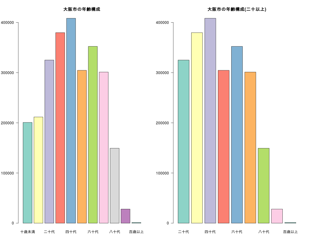
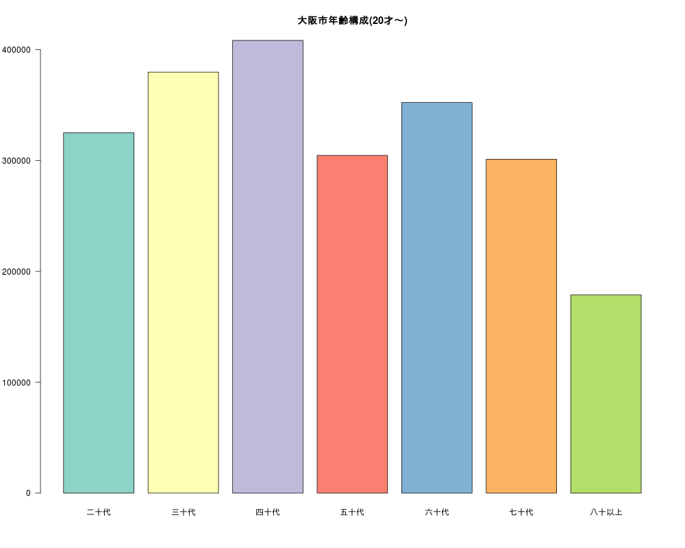
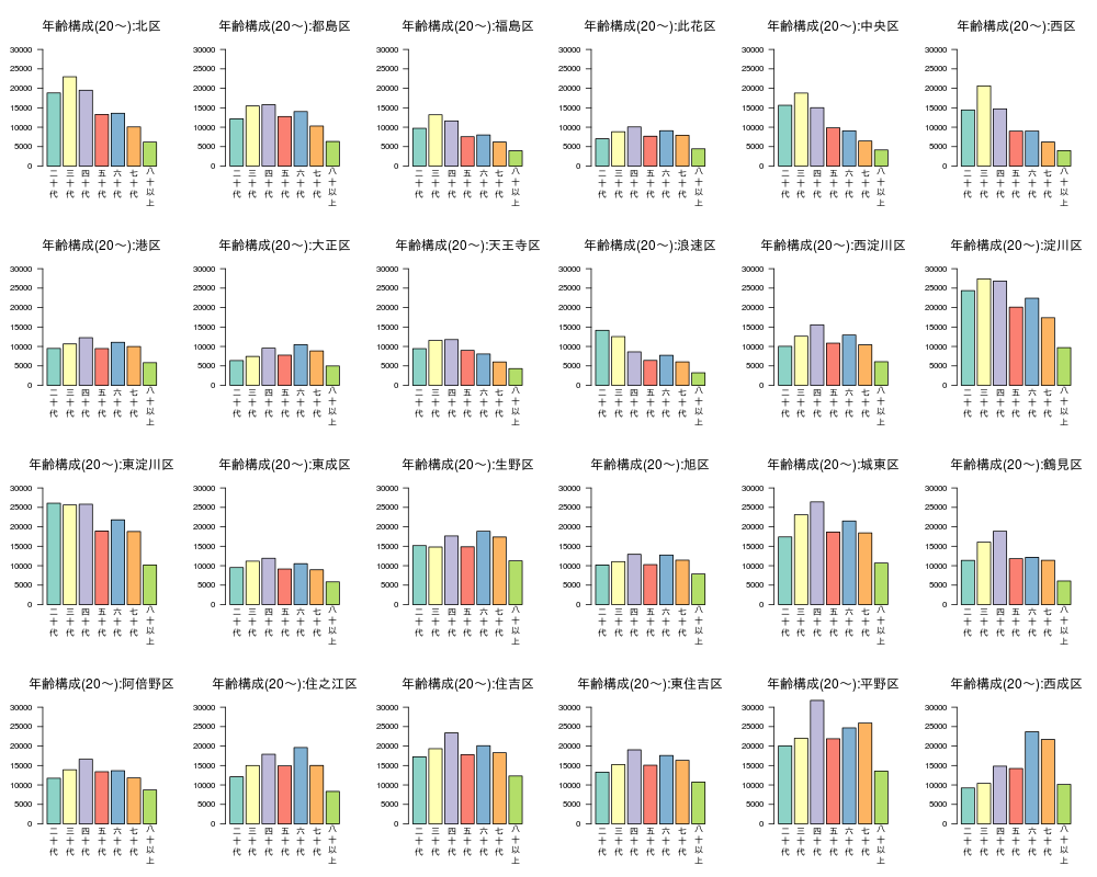
大阪市棒グラフ

大阪市の各区の年齢構成

(参考・使用したデータ等)
大阪市における特別区の設置についての投票
区ごとの年齢構成

使用するOS、Rのバージョンによってデータを取り込む命令が異なる。
使うデータはあらかじめダウンロードしておくのが一番よい。

ここではOSはzorin。RのバージョンR3.1.2

1
2
3
4
5
6
7
8
9
10
11
#大阪市の各区の年齢構成
#URLスキームがhttpsの場合read.csvでは読み込めないこともあり。
#方法1 read.csv
#age<-read.csv("https://raw.githubusercontent.com/yutannihilation/osaka_age_composition/master/osaka_age_composition.csv",fileEncoding="UTF-8")
#方法2 downloaderパッケージのdownload
library(downloader)
download("https://raw.githubusercontent.com/yutannihilation/osaka_age_composition/master/osaka_age_composition.csv","age.csv")
age<-read.csv("age.csv",fileEncoding="UTF-8")
#方法3 ダウンロードしてから読み込む。
#https://raw.githubusercontent.com/yutannihilation/osaka_age_composition/master/osaka_age_composition.csv からDL。作業ディレクトリに保存
#age = read.csv("osaka_age_composition.csv",fileEncoding="UTF-8")

棒グラフ

1
2
3
4
5
6
7
8
9
10
11
12
13
14
15
16
17
18
19
20
21
22
library(RColorBrewer)
options(scipen=10)
#層別集計作業
age$class<- cut(age$age,breaks=c(seq(0,100,10),101), right=F, ordered_result=TRUE)
head(age);tail(age)
#by(age2$total, age$class,sum)
#tapply(age2$total, age$class,sum)
aggregate(total~class,age,sum)
#png("osaka03.png",width=1000,height=800)
par(mfrow=c(1,2))
barplot(aggregate(total~class,age,sum)$total,
names.arg=c("十歳未満","十代","二十代","三十代","四十代","五十代","六十代","七十代","八十代","九十代","百歳以上"),col=brewer.pal(10, "Set3"),las=1)
title("大阪市の年齢構成")
#
#二十以上
#
age2 <- subset(age, class!="[0,10)" & class!="[10,20)", select=c(class,district,total))
barplot(aggregate(total~class,age2,sum)$total,
names.arg=c("二十代","三十代","四十代","五十代","六十代","七十代","八十代","九十代","百歳以上"),col=brewer.pal(8, "Set3"),las=1)
title("大阪市の年齢構成(二十以上)")
par(mfrow=c(1,1))
#dev.off()

1
2
3
4
5
6
7
8
9
10
11
#library(RColorBrewer)
#options(scipen=10)
#層別集計作業(80歳以上まとめた)
age$class<- cut(age$age,breaks=c(seq(0,80,10),101), right=F, ordered_result=TRUE)
#head(age);tail(age)
age2 <- subset(age, class!="[0,10)" & class!="[10,20)", select=c(class,district,total))
#png("osaka04.png",width=1000,height=800)
barplot(aggregate(total~class,age2,sum)$total,
names.arg=c("二十代","三十代","四十代","五十代","六十代","七十代","八十以上"),col=brewer.pal(8, "Set3"),las=1)
title("大阪市年齢構成(20才~)")
#dev.off()

大阪市各区の年齢構成
グラフの最大値 : max(xtabs(total~class+district,age2)))

1
2
3
4
5
6
7
8
9
10
11
12
13
14
15
16
17
18
19
20
21
22
23
#縦書き関数を定義
tate <- function(x){
x<-as.vector(x)
for(i in 1:length(x)){
xx<-chartr("ー", "|",x[i])
xx<-unlist(strsplit(xx,""))
x[i]<-paste(xx,collapse= "\n")
}
return(x)
}
# 層別グラフ(画面24分割)
#png("osaka05.png",width=1000,height=800)
par(mfrow=c(4,6))
for(i in unique(age2[,"district"])){
df= subset(age2,district==i)
b<-barplot(aggregate(total~class,df,sum)$total,names.arg=NA,
horiz=F,las=1,cex.names=0.8,col=brewer.pal(8, "Set3"),ylim=c(0,max(xtabs(total~class+district,age2))))
text(b[1:7,],-1000,labels=tate(c("二十代","三十代","四十代","五十代","六十代","七十代","八十以上")),
srt=0,col=c(rep("black",30),"red",rep("black",16)),xpd=TRUE,pos=1)
mtext(side=3, line=1, text=paste("年齢構成(20~):",i,"区",sep=""))
}
par(mfrow=c(1,1))
#dev.off()