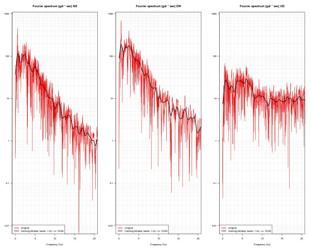
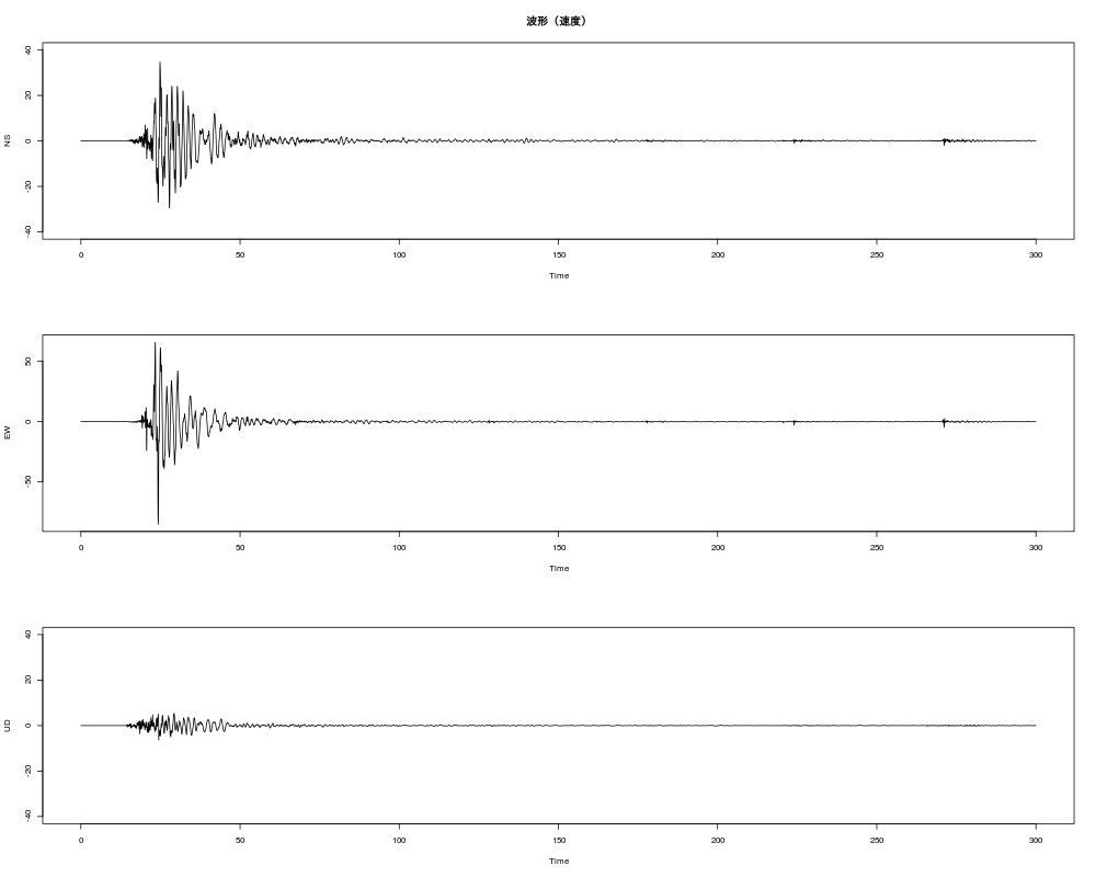
gridx=c(seq(0,20,1)) gridy=c(seq(0.001,0.009,0.001),seq(0.01,0.09,0.01),seq(0.1,0.9,0.1),seq(1,9,1),seq(10,90,10),seq(100,900,100),seq(1000,10000,1000)) par(mfrow=c(1,3)) plot(resNS$frq,resNS$fs1,type="l",log="y",las=1,col="red",xlab="Frequency (Hz)",ylab="",yaxt="n", panel.first = abline(v=gridx,h=gridy,col="lightgray",lty ="dotted"),xlim=c(0,20),ylim=c(1e-2,7e+2)) axis(2,c(0.00001,0.0001,0.001,0.01,0.1,1,10,100,1000,10000), c("0.00001","0.0001","0.001","0.01","0.1","1","10","100","1000","10000"),las=1) lines(resNS$frq,resNS$fs2,col="black",lwd=2) title("Fourier spectrum (gal * sec) NS") legend( "bottomleft", c("Original",paste("Hanning Window :band=",band,"Hz : n=",n)), col = c("red","black"), lty = 1, lwd = 2, bg = "white" ) plot(resEW$frq,resEW$fs1,type="l",log="y",las=1,col="red",xlab="Frequency (Hz)",ylab="",yaxt="n", panel.first = abline(v=gridx,h=gridy,col="lightgray",lty ="dotted"),xlim=c(0,20),ylim=c(1e-2,7e+2)) axis(2,c(0.00001,0.0001,0.001,0.01,0.1,1,10,100,1000,10000), c("0.00001","0.0001","0.001","0.01","0.1","1","10","100","1000","10000"),las=1) lines(resEW$frq,resEW$fs2,col="black",lwd=2) title("Fourier spectrum (gal * sec) EW") legend( "bottomleft", c("Original",paste("Hanning Window :band=",band,"Hz : n=",n)), col = c("red","black"), lty = 1, lwd = 2, bg = "white" ) plot(resUD$frq,resUD$fs1,type="l",log="y",las=1,col="red",xlab="Frequency (Hz)",ylab="",yaxt="n", panel.first = abline(v=gridx,h=gridy,col="lightgray",lty ="dotted"),xlim=c(0,20),ylim=c(1e-2,7e+2)) axis(2,c(0.00001,0.0001,0.001,0.01,0.1,1,10,100,1000,10000), c("0.00001","0.0001","0.001","0.01","0.1","1","10","100","1000","10000"),las=1) lines(resUD$frq,resUD$fs2,col="black",lwd=2) title("Fourier spectrum (gal * sec) UD") legend( "bottomleft", c("Original",paste("Hanning Window :band=",band,"Hz : n=",n)), col = c("red","black"), lty = 1, lwd = 2, bg = "white" ) par(mfrow=c(1,1))
|