21世紀の資本グラフ4

Quandl、xts、stringr、grid、plotrix、RColorBrewer、knitr パッケージ

「21世紀の資本」のデータが公開されてるのでRを使ってグラフ化してみます。
(グラフもすでに公開されているのであまり意味はありません。)
(参考)
Piketty Codes
『21世紀の資本』日本語版サポートページ

Chapter 4: From Old Europe to the New World

Capital in Germany, 1870-2010
1
2
3
4
5
6
7
8
9
10
11
12
13
14
15
16
17
18
19
20
21
22
23
24
25
26
27
28
29
30
31
library(xts)
library(Quandl)
TS4_1<-Quandl("PIKETTY/TS4_1")
#並べ替え
sortlist <- order(TS4_1[,1])
dat <- TS4_1[sortlist,]
TS4_1<-dat
rownames(TS4_1) <- c(1:nrow(TS4_1))
#save("TS4_1", file="TS4_1.dat")
#load("TS4_1.dat")
##### TS4_1 #####
#1 Year 年
#2 National capital Wn 国民資本
#3 incl. Land 土地
#4 incl. Housing 住宅
#5 incl. Other domestic capital assets その他の国内資本資産
#6 incl. Net foreign capital 純外国資本
#7 Public capital Wg 公的資本
#8 incl. Public assets 公的資産
#9 incl. Public debt 公的債務
#10 Private capital W 民間資本
#11 Land
#12 Housing + land
#13 Land + housing + other + NFA
#14 Net foreign assets
library(knitr)
library(stringr)
library("plotrix")
library(RColorBrewer)
#表 str_sub関数で○○年だけを抽出
kable(data.frame(year=str_sub(TS4_1[,1], start=1, end=4),TS4_1[,3:6]))
year incl..Land incl..Housing incl..Other.domestic.capital.assets incl..Net.foreign.capital
1870 281.63284 82.82973 319.9440 6.41051
1890 174.23696 100.50671 303.4437 47.47687
1910 144.40640 120.31942 339.6198 44.10692
1930 48.10225 63.89285 253.2152 -11.12660
1950 27.41280 60.45407 146.3691 -0.85175
1970 13.47624 127.85849 164.4385 7.56632
1990 4.67917 181.33622 158.0899 11.01127
2000 3.21160 212.90213 153.6467 17.75637
2010 3.36156 231.28869 140.9178 38.73830
1
2
3
4
5
6
7
8
9
#png("PikettyTS4_1A.png",width=1000,height=800)
#stringrパッケージのstr_sub関数を使う
#stackpoly(TS4_1[,3:6],ylim=c(0,800),axis4=F,main="Capital in Germany, 1870-2010",col=brewer.pal(4,"Pastel1"),
#xaxlab=str_sub(TS4_1[,1], start=1, end=4),border="gray36",staxx=F,stack=TRUE)
stackpoly(TS4_1[,3:6],ylim=c(0,800),axis4=F,main="Capital in Germany, 1870-2010",
col=c("#FBB4AE","#B3CDE3",rgb(204/255,235/255,197/255,alpha=0.5),"#DECBE4"),
xaxlab=str_sub(TS4_1[,1], start=1, end=4),border="gray36",staxx=F,stack=TRUE)
boxed.labels(c(2.5,2.5,2.5,2.5),c(100,200,400,620),c("土地","住宅","その他国内資本","純外国資本"),border=F,bg=NA,col="gray20",cex=2)
#dev.off()

Capital in The United States, 1870-2010
1
2
3
4
5
6
7
8
9
10
11
12
13
14
15
16
17
18
19
20
21
22
23
24
25
26
27
28
29
library(xts)
library(Quandl)
TS4_2<-Quandl("PIKETTY/TS4_2")
#並べ替え
sortlist <- order(TS4_2[,1])
dat <- TS4_2[sortlist,]
TS4_2<-dat
rownames(TS4_2) <- c(1:nrow(TS4_2))
#save("TS4_2", file="TS4_2.dat")
#load("TS4_2.dat")
##### TS4_2 #####
#1 Year 年
#2 National capital Wn 国民資本
#3 incl. Land 土地
#4 incl. Housing 住宅
#5 incl. Other domestic capital assets その他の国内資本資産
#6 incl. Net foreign capital 純外国資本
#7 Public capital Wg 公的資本
#8 incl. Public assets 公的資産
#9 incl. Public debt 公的債務
#10 Private capital W 民間資本
#11 Slaves
#12 National capital incl. Slaves
library(knitr)
library(stringr)
library("plotrix")
library(RColorBrewer)
#表
kable(data.frame(year=str_sub(TS4_2[,1], start=1, end=4),TS4_2[,3:6]))
year incl..Land incl..Housing incl..Other.domestic.capital.assets incl..Net.foreign.capital
1770 165.748674 82.87434 77.15887 -12.530072
1810 120.370370 62.50000 121.29630 -14.814815
1850 121.757499 60.83650 166.70891 -9.294466
1880 88.678819 110.40807 238.43444 -15.464960
1910 101.943092 104.52393 290.02164 -6.774699
1920 59.107972 102.54877 258.20950 12.405313
1930 46.458888 151.22434 317.86396 13.205538
1950 23.738537 145.63395 205.05334 5.357332
1970 19.052292 150.60826 225.87795 4.608742
1990 8.504568 174.32180 244.35734 -8.205476
2010 11.567527 182.48670 262.12925 -25.425782
1
2
3
4
5
6
7
8
9
#png("PikettyTS4_2A.png",width=1000,height=800)
#stringrパッケージのstr_sub関数を使う
#stackpoly(TS4_2[,3:6],ylim=c(0,800),axis4=F,main="Capital in The United States, 1870-2010",col=brewer.pal(4,"Pastel1"),
#xaxlab=str_sub(TS4_2[,1], start=1, end=4),border="gray36",staxx=F,stack=TRUE)
stackpoly(TS4_2[,3:6],ylim=c(0,800),axis4=F,main="Capital in The United States, 1870-2010",
col=c("#FBB4AE","#B3CDE3",rgb(204/255,235/255,197/255,alpha=0.5),"#DECBE4"), #rgb(222/255,203/255,228/255,alpha=1)
xaxlab=str_sub(TS4_2[,1], start=1, end=4),border="gray36",staxx=F,stack=TRUE)
boxed.labels(c(4,4,4,7),c(50,160,280,510),c("土地","住宅","その他国内資本","純外国資本"),border=F,bg=NA,col="gray20",cex=2)
#dev.off()

Capital in Canada, 1860-2010
1
2
3
4
5
6
7
8
9
10
11
12
13
14
15
16
17
18
19
20
21
22
23
24
25
26
27
28
29
30
31
library(xts)
library(Quandl)
TS4_3<-Quandl("PIKETTY/TS4_3")
#並べ替え
sortlist <- order(TS4_3[,1])
dat <- TS4_3[sortlist,]
TS4_3<-dat
rownames(TS4_3) <- c(1:nrow(TS4_3))
#save("TS4_3", file="TS4_3.dat")
#load("TS4_3.dat")
##### TS4_3 #####
#1 Year 年
#2 National capital Wn 国民資本
#3 incl. Land 土地
#4 incl. Housing 住宅
#5 incl. Other domestic capital assets その他の国内資本資産
#6 incl. Net foreign capital 純外国資本
#7 Public capital Wg 公的資本
#8 incl. Public assets 公的資産
#9 incl. Public debt 公的債務
#10 Private capital W 民間資本
#11 Land
#12 Housing + land
#13 Land + housing + other + NFA
#14 Net foreign assets
library(knitr)
library(stringr)
library("plotrix")
library(RColorBrewer)
#表
kable(data.frame(year=str_sub(TS4_3[,1], start=1, end=4),TS4_3[,3:6]))
year incl..Land incl..Housing incl..Other.domestic.capital.assets incl..Net.foreign.capital
1860 195.39816 71.57442 157.4637 -40.00000
1890 125.68306 93.52159 298.2817 -128.70133
1910 101.13513 108.90479 318.8610 -115.53749
1920 66.26533 128.73826 354.7880 -115.89917
1950 15.29589 133.16422 216.8417 -32.99774
1970 16.83251 121.25102 183.8464 -36.94733
1980 15.02114 128.13300 179.0969 -44.61274
1990 10.88013 150.85410 182.4289 -44.87069
2000 11.89124 171.60875 188.1887 -10.24872
2010 14.24536 207.92929 195.0333 -12.23513
1
2
3
4
5
6
7
8
9
10
11
#png("PikettyTS4_3A.png",width=1000,height=800)
#stringrパッケージのstr_sub関数を使う
#stackpoly(TS4_3[,3:6],ylim=c(0,800),axis4=F,main="Capital in Canada, 1860-2010",col=brewer.pal(4,"Pastel1"),
#xaxlab=str_sub(TS4_3[,1], start=1, end=4),border="gray36",staxx=F,stack=TRUE)
#boxed.labels(c(2,3,3,2),c(80,150,400,620),c("土地","住宅","その他国内資本",""),border=F,bg=NA,col="gray20",cex=2)
stackpoly(TS4_3[,3:6],ylim=c(0,800),axis4=F,main="Capital in Canada, 1860-2010",
col=c("#FBB4AE","#B3CDE3",rgb(204/255,235/255,197/255,alpha=0.5),"#DECBE4"),
xaxlab=str_sub(TS4_3[,1], start=1, end=4),border="gray36",staxx=F,stack=TRUE)
boxed.labels(c(2,3,3,3),c(80,150,350,470),c("土地","住宅","その他国内資本","純外国資本(マイナス)"),border=F,bg=NA,
col=c("gray20","gray20","gray20","red"),cex=2)
#dev.off()

National, Public and Private Capital in Europe and in the United States, 1870-2010
1
2
3
4
5
6
7
8
9
10
11
12
13
14
15
16
17
18
19
20
21
22
23
24
25
26
27
28
29
30
library(xts)
library(Quandl)
TS4_5<-Quandl("PIKETTY/TS4_5")
#並べ替え
sortlist <- order(TS4_5[,1])
dat <- TS4_5[sortlist,]
TS4_5<-dat
rownames(TS4_5) <- c(1:nrow(TS4_5))
#save("TS4_5", file="TS4_5.dat")
#load("TS4_5.dat")
TS4_5.xts<-as.xts(read.zoo(TS4_5))
#png(file="TS4_5_1.png",width =1000, height =800)
par(mfrow=c(3,1),mar = c(2,4,3,11))
#Private Capital
TS4_5Private.xts<-TS4_5.xts[,1:4]
plot.zoo(TS4_5Private.xts,main="Private Capital in Europe and in the United States, 1870-2010",plot.type="single",
col=1:ncol(TS4_5Private.xts),lwd=2,xlab="年",ylab="",las=1)
axis(4,TS4_5Private.xts[nrow(TS4_5Private.xts),],colnames(TS4_5Private.xts),col.axis="black" ,las=1)
#Nationa Capital
TS4_5National.xts<-TS4_5.xts[,6:9]
plot.zoo(TS4_5National.xts,main="Nationa Capital in Europe and in the United States, 1870-2010",plot.type="single",
col=1:ncol(TS4_5National.xts),lwd=2,xlab="年",ylab="")
axis(4,TS4_5National.xts[nrow(TS4_5National.xts),],colnames(TS4_5National.xts),col.axis="black" ,las=1)
#Public Capital
TS4_5Public.xts<-TS4_5.xts[,11:14]
plot.zoo(TS4_5Public.xts,main="Public Capital in Europe and in the United States, 1870-2010",plot.type="single",
col=1:ncol(TS4_5Public.xts),lwd=2,xlab="年",ylab="")
axis(4,TS4_5Public.xts[nrow(TS4_5Public.xts),],colnames(TS4_5Public.xts),col.axis="black" ,las=1)
par(mfrow=c(1,1))
#dev.off()

xtsplot関数修正(2015/3/1)

coredata() -> data.frame(coredata())とする必要あり!!

1
2
3
4
5
6
7
8
9
10
11
12
13
14
15
16
17
18
19
20
21
22
23
24
25
26
27
#ggplot2パッケージを使う
#手順を繰り返すのが面倒。xtsplot関数を定義する
##############
xtsplot<-function(x) {
library(ggplot2)
library(reshape2)
#最終データの降順に並べ替える
#凡例を降順に並べるため
d0<-data.frame(coredata(x))
y<-d0[order(d0[nrow(d0),], decreasing = TRUE)]
data<-data.frame(date=index(x),y)
data.melt <- melt(data,id.vars=c("date"),measure.vars=c(colnames(data[2:ncol(data)])))
ggplot(data.melt, aes(x=as.Date(date),y=value,colour=variable,group=variable)) + geom_line(size = 1.5,linetype=1,alpha = 1)+labs(x="", y="")
}
#############
#定義したxtsplot関数を使ってプロット
library(grid)
#png(file="TS4_5_2.png",width =1000, height =800)
grid.newpage() #空の画面を作る
pushViewport(viewport(layout=grid.layout(3,))) #画面を区切る(今回は2行2列の4分割)
p1<-xtsplot(TS4_5Private.xts) + labs(title="Private Capital in Europe and in the United States, 1870-2010")
p2<-xtsplot(TS4_5Public.xts) + labs(title="Public Capital in Europe and in the United States, 1870-2010")
p3<-xtsplot(TS4_5National.xts) + labs(title="National Capital in Europe and in the United States, 1870-2010")
print(p1, vp=viewport(layout.pos.row=1, layout.pos.col=1)) #1行目
print(p2, vp=viewport(layout.pos.row=2, layout.pos.col=1)) #2行目
print(p3, vp=viewport(layout.pos.row=3, layout.pos.col=1)) #3行目
#dev.off()

グラフを並べて、線の色で国を区別したいときにはいい方法ではない。

並べ替えをしない
1
2
3
4
5
6
7
8
9
10
11
12
13
14
15
16
17
18
19
xtsplot2<-function(x) {
library(ggplot2)
library(reshape2)
data<-data.frame(date=index(x),coredata(x))
data.melt <- melt(data,id.vars=c("date"),measure.vars=c(colnames(data[2:ncol(data)])))
ggplot(data.melt, aes(x=as.Date(date),y=value,colour=variable,group=variable)) + geom_line(size = 1.5,linetype=1,alpha = 1)+labs(x="", y="")
}
#############
library(grid)
#png(file="TS4_5_3.png",width =1000, height =800)
grid.newpage()
pushViewport(viewport(layout=grid.layout(3,)))
p1<-xtsplot2(TS4_5Private.xts) + labs(title="Private Capital in Europe and in the United States, 1870-2010")
p2<-xtsplot2(TS4_5Public.xts) + labs(title="Public Capital in Europe and in the United States, 1870-2010")
p3<-xtsplot2(TS4_5National.xts) + labs(title="National Capital in Europe and in the United States, 1870-2010")
print(p1, vp=viewport(layout.pos.row=1, layout.pos.col=1))
print(p2, vp=viewport(layout.pos.row=2, layout.pos.col=1))
print(p3, vp=viewport(layout.pos.row=3, layout.pos.col=1))
#dev.off()

以下はグラフは省略

Capital in Britain, 1700-2010
1
2
3
4
5
6
7
8
9
10
11
12
13
14
15
16
17
18
19
20
21
22
23
24
25
26
27
28
29
30
31
32
33
34
35
36
37
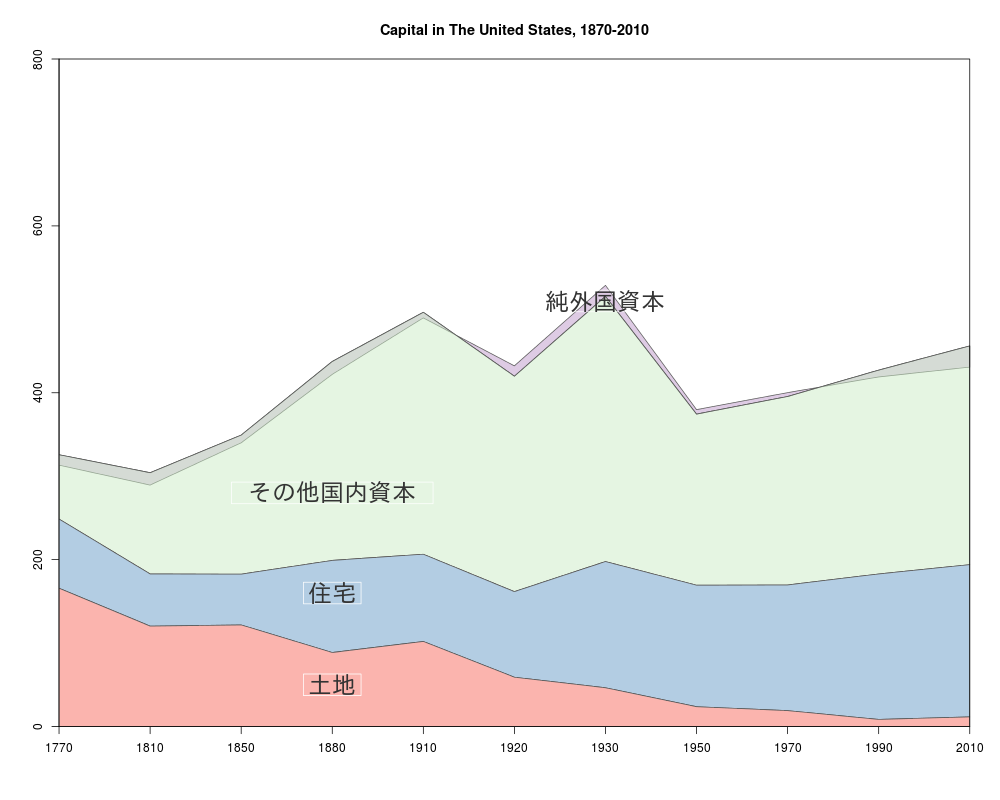
library(xts)
library(Quandl)
T3_1<-Quandl("PIKETTY/T3_1")
#並べ替え
sortlist <- order(T3_1[,1])
dat <- T3_1[sortlist,]
T3_1<-dat
rownames(T3_1) <- c(1:nrow(T3_1))
#save("T3_1", file="T3_1.dat")
#load("T3_1.dat")
##### T3_1 #####
#1 Year 年
#2 National capital Wn 国民資本
#3 incl. Land 土地
#4 incl. Housing 住宅
#5 incl. Other domestic capital assets その他の国内資本資産
#6 incl. Net foreign capital 純外国資本
#7 Public capital Wg 公的資本
#8 incl. Public assets 公的資産
#9 incl. Public debt 公的債務
#10 Private capital W 民間資本
library(knitr)
library(stringr)
library("plotrix")
library(RColorBrewer)
#表
kable(data.frame(year=str_sub(T3_1[,1], start=1, end=4),T3_1[,3:6]))
#png("Piketty3_1A.png",width=1000,height=800)
stackpoly(T3_1[,3:6],ylim=c(0,800),axis4=F,main="イギリスの資本 1700-2010年",
col=c("#FBB4AE","#B3CDE3",rgb(204/255,235/255,197/255,alpha=0.5),"#DECBE4"),
xaxlab=str_sub(T3_1[,1], start=1, end=4),border="gray36",staxx=F,stack=TRUE)
#boxed.labels(3,180,"土地",border=F,bg=NA,col="gray20")
#boxed.labels(4,300,"住宅",border=F,bg=NA,col="gray20")
#boxed.labels(4,500,"その他国内資本",border=F,bg=NA,col="gray20")
#boxed.labels(5.4,620,"純外国資本",border=F,bg=NA,col="gray20")
boxed.labels(c(3,4,4,5.4),c(180,300,500,620),c("土地","住宅","その他国内資本","純外国資本"),border=F,bg=NA,col="gray20",cex=2)
#dev.off()
Capital in the France, 1700-2010
1
2
3
4
5
6
7
8
9
10
11
12
13
14
15
16
17
18
19
20
21
22
23
24
25
26
27
28
29
30
31
32
33
34
35
library(xts)
library(Quandl)
T3_2<-Quandl("PIKETTY/T3_2")
#並べ替え
sortlist <- order(T3_2[,1])
dat <- T3_2[sortlist,]
T3_2<-dat
rownames(T3_2) <- c(1:nrow(T3_2))
#save("T3_2", file="T3_2.dat")
#load("T3_2.dat")
##### T3_2 #####
#1 Year 年
#2 National capital Wn 国民資本
#3 incl. Land 土地
#4 incl. Housing 住宅
#5 incl. Other domestic capital assets その他の国内資本資産
#6 incl. Net foreign capital 純外国資本
#7 Public capital Wg 公的資本
#8 incl. Public assets 公的資産
#9 incl. Public debt 公的債務
#10 Private capital W 民間資本
#11 incl. private assets 民間資産
#12 incl. private debt 民間負債
library(knitr)
library(stringr)
library("plotrix")
library(RColorBrewer)
#表
kable(data.frame(year=str_sub(T3_2[,1], start=1, end=4),T3_2[,3:6]))
#png("Piketty3_2A.png",width=1000,height=800)
stackpoly(T3_2[,3:6],ylim=c(0,800),axis4=F,main="フランスの資本 1700-2010年",
col=c("#FBB4AE","#B3CDE3",rgb(204/255,235/255,197/255,alpha=0.5),"#DECBE4"),
xaxlab=str_sub(T3_2[,1], start=1, end=4),border="gray36",staxx=F,stack=TRUE)
boxed.labels(c(3,4,4,6),c(180,400,600,670),c("土地","住宅","その他国内資本","純外国資本"),border=F,bg=NA,col="gray20",cex=2)
#dev.off()