巡回セールスマン問題Concorde法

巡回セールスマン問題 method=”concorde”


solve_TSP( x, method, control )のアルゴリズムに“concorde”, “linkern” を使用する。
(準備)
The Traveling Salesman ProblemからSolver パッケージをダウンロード
OSはzorinOSを使っているので
concorde-linux,linkern-linuxをDL ー> 解凍 ー> 適当なフォルダ(ここでは/home/user)に移動
ー> 「ファイルのプロパティ」で実行権限を「誰でも」にする
download informationに「 ~are available for academic research use」とあるので使用する目的によっては許可が必要。

1
2
3
4
5
6
7
8
9
10
11
12
13
14
15
16
17
18
19
20
21
22
23
24
25
26
27
28
29
30
31
32
33
34
library(maptools)
library(rgdal)
library(sp)
library(TSP)
concorde_path("/home/user")
#shapeファイル、sa.csvのフォルダ名ファイル名は環境によって違います。
jpn<-readShapeSpatial("/home/user/R/work/JPN/JPN_adm0.shp")
sc <- read.table("/home/user/R/work/sc.csv", header=TRUE, sep=",", na.strings="NA", dec=".", strip.white=TRUE)
names(sc)<-c("name","address","lat","lon")
#spDistsN1で距離を計算。距離行列を作成。
nr<-nrow(sc)
distance = matrix(0, nr, nr)
for(i in 1:(nr-1)){
sc_i = sc[i,]
loc_i = cbind(sc_i$lon, sc_i$lat)
for(j in (i+1):nr){
sc_j = sc[j,]
loc_j = cbind(sc_j$lon,sc_j$lat)
route_ij = spDistsN1(loc_i, loc_j,longlat=TRUE)
distance[i,j] = distance[j,i] = route_ij
}
}
rownames(distance)<-sc$name
colnames(distance)<-sc$name
#solve_TSP関数のすべてのmethodを使って最短経路を計算。パラメータはdefault
methods <- c( "nearest_insertion", "cheapest_insertion",
"farthest_insertion", "arbitrary_insertion",
"nn", "repetitive_nn", "2-opt","concorde","linkern")
tours <- lapply(methods, FUN = function(m) solve_TSP(TSP(ATSP(distance)), method = m))
names(tours) <- methods
tour_lengths <- c(sapply(tours, FUN = attr, "tour_length"))
#最短のmethodを確認
tour_lengths
dotchart( tour_lengths)

nearest_insertion cheapest_insertion farthest_insertion
6383.965 6350.778 6268.405
arbitrary_insertion nn repetitive_nn
6216.112 7459.273 6950.645
2-opt concorde linkern
6197.878 6082.051 6082.051

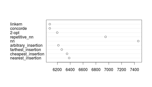
‘2-opt’も健闘したけど’concorde’と’linkern’(3回やって3回とも6082.051km)とは100km以上の差

methodは’concorde’

1
2
3
4
5
6
7
8
9
10
11
12
13
14
15
16
17
shortest<-tours$'concorde'
shortest
#経路1番から6番までを表示
order<-as.integer(shortest)
#データscを経路順に並べ替え
sctsp <- sc[ order,]
proj4string(jpn)="+proj=longlat"
plot(jpn, xlim=c(127.5, 149), ylim=c(26, 45.5),xlab="", ylab="",col="#d0e0ff",axes=F,border="grey")
points(sctsp$lon, sctsp$lat,col="blue",pch=16,cex=0.8)
#nr<-nrow(sc)
for(i in 1:(nr-1)){
sc_i = sctsp[i,]
sc_j = sctsp[(i+1),]
segments(sc_i$lon,sc_i$lat,sc_j$lon,sc_j$lat,lwd = 1, col = "red")
}
segments(sctsp[nr,]$lon,sctsp[nr,]$lat,sctsp[1,]$lon,sctsp[1,]$lat,lwd=1,col="red")
title(main="学習センター最短直線経路(RのTSPパッケージで得た近似解の一例)")

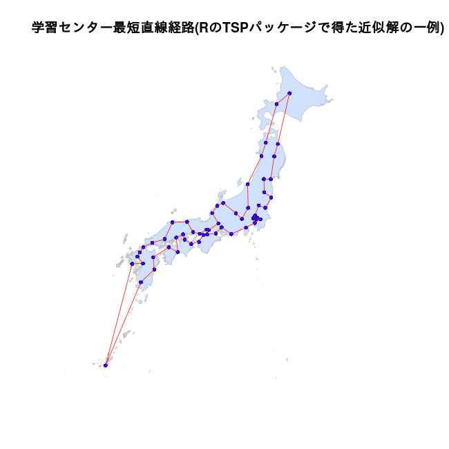
  • 「メタヒューリスティクス2」の経路とは中国地方・四国地方の回りかたが異なる。