Oct 13 2014

非線形計画法2

第13章非線形計画法2

p.175 例2

$$\begin{aligned} z=&\sqrt{(x_1-1)^2+(x_2-12)^2}+\sqrt{(x_1-4)^2+(x_2-14)^2}+\sqrt{(x_1-15)^2+(x_2-10)^2}\\ &+\sqrt{(x_1-11)^2+(x_2-2)^2}+\sqrt{(x_1-5)^2+(x_2-5)^2} \end{aligned}$$

model<-function(x) {
return( sqrt((x[1]-1)^2+(x[2]-12)^2)+sqrt((x[1]-4)^2+(x[2]-14)^2)+sqrt((x[1]-15)^2+(x[2]-10)^2)+sqrt((x[1]-11)^2+(x[2]-2)^2)+sqrt((x[1]-5)^2+(x[2]-5)^2)) 
}
x0 <- c(0.7, 0.1) # xの初期値

optim関数

1
2
3

res1 <- optim(x0, model) # Nelder and Mead シンプレックス法
res2 <- optim(x0, model, method="BFGS") # 準ニュートン法 (BFGS法)
res1;res2

res1;res2

$par
[1] 6.353805 8.163534

$value
[1] 32.87839

$counts
function gradient
85 NA

$convergence
[1] 0

$message
NULL

$par
[1] 6.353591 8.162658

$value
[1] 32.87839

$counts
function gradient
11 8

$convergence
[1] 0

$message
NULL

nlm関数

1 2	res <- nlm(model,x0,print.level=2) res

$minimum
[1] 32.87839

$estimate
[1] 6.353552 8.162883

$gradient
[1] 2.270229e-07 1.321352e-06

$code
[1] 1

$iterations
[1] 8

BBパッケージ

library(BB)
#Derivative-Free Spectral Approach for solving nonlinear systems of equations
#ans<-dfsane(x0,model)
#ans
#A strategy using different Barzilai-Borwein steplengths to solve a nonlinear system of equations.
#ans<-BBsolve(x0,model)
#ans
#A strategy using different Barzilai-Borwein steplengths to optimize a nonlinear objective function subject to box constraints.
ans1<-BBoptim(x0,model)
#Spectral projected gradient method for large-scale optimization with simple constraints.
ans2<-spg(x0,model)
ans1;ans2

$par
[1] 6.353546 8.162880

$value
[1] 32.87839

$gradient
[1] 4.689582e-06

$fn.reduction
[1] 27.69725

$iter
[1] 8

$feval
[1] 10

$convergence
[1] 0

$message
[1] “Successful convergence”

$cpar
method M
2 50

$par
[1] 6.353540 8.162878

$value
[1] 32.87839

$gradient
[1] 8.100187e-06

$fn.reduction
[1] 27.69725

$iter
[1] 8

$feval
[1] 10

$convergence
[1] 0

$message
[1] “Successful convergence”

滑降シンプレックス法

1 2	library(adagio) nelmin(model,x0)

$xmin
[1] 6.353555 8.162882

$fmin
[1] 32.87839

$fcount
[1] 223

$restarts
[1] 0

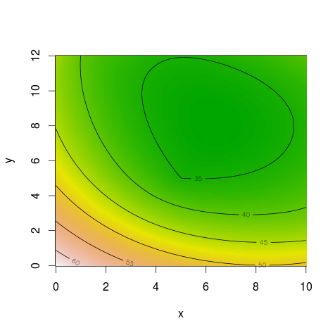
（おまけ）関数の視覚化

x <- seq(0,10,length=200)
y <- seq(0,12,length=200)
f<- function(x,y) { 
  sqrt((x-1)^2+(y-12)^2)+sqrt((x-4)^2+(y-14)^2)+sqrt((x-15)^2+(y-10)^2)+sqrt((x-11)^2+(y-2)^2)+sqrt((x-5)^2+(y-5)^2) 
}
#XとYの組み合わせに対して関数fを適用する
z <- outer(x,y,f)
image(x, y, z, col = terrain.colors(100),axes=T)
contour(x,y,z,add=T)

第13章 非線形計画法2

p.175 例2

第13章非線形計画法2