最短路問題

問題解決の数理 第4章 ネットワーク計画法1

線形計画問題として解く

最小化

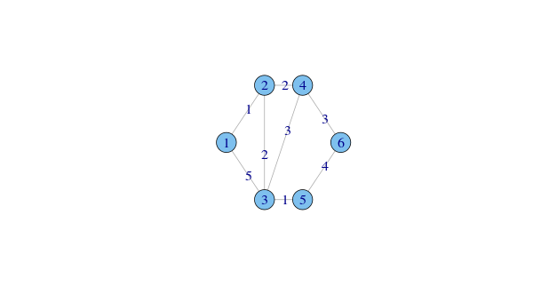
$$\begin{aligned} &z=x_{12}+x_{21}+5x_{13}+5x_{31}+2x_{23}+2x_{32}+2x_{24}+2x_{42}\\ &+3x_{34}+3x_{43}+x_{35}+x_{53}+3x_{46}+3x_{64}+4x_{56}+4x_{65} \end{aligned}$$

制約条件

$$\begin{aligned} &x_{12}-x_{21}+x_{13}-x_{31}+0x_{23}+0x_{32}+0x_{24}+0x_{42}\\ &+0x_{34}+0x_{43}+0x_{35}+0x_{53}+0x_{46}+0x_{64}+0x_{56}+0x_{65}=1\\ &0x_{12}+0x_{21}+0x_{13}+0x_{31}+0x_{23}+0x_{32}+0x_{24}+0x_{42}\\ &+0x_{34}+0x_{43}-x_{35}+x_{53}+0x_{46}+0x_{64}+x_{56}-x_{65}=-1\\ &-x_{12}+x_{21}+0x_{13}+0x_{31}+x_{23}-x_{32}+x_{24}-x_{42}\\ &+0x_{34}+0x_{43}+0x_{35}+0x_{53}+0x_{46}+0x_{64}+0x_{56}+0x_{65}=0\\ &0x_{12}+0x_{21}-x_{13}+x_{31}-x_{23}+x_{32}+0x_{24}+0x_{42}\\ &+x_{34}-x_{43}+x_{35}-x_{53}+0x_{46}+0x_{64}+0x_{56}+0x_{65}=0\\ &0x_{12}+0x_{21}+0x_{13}+0x_{31}+0x_{23}+0x_{32}-x_{24}+x_{42}\\ &-x_{34}+x_{43}+0x_{35}+0x_{53}+x_{46}-x_{64}+0x_{56}+0x_{65}=0\\ &0x_{12}+0x_{21}+0x_{13}+0x_{31}+0x_{23}+0x_{32}+0x_{24}+0x_{42}\\ &+0x_{34}+0x_{43}+0x_{35}+0x_{53}-x_{46}+x_{64}-x_{56}+x_{65}=0\\ \end{aligned}$$

$$x_{ij}\geq0 for (i,j) \in E$$

library(linprog)
# 最小化(maximum=F)
cvec<-c(1,1,5,5,2,2,2,2,3,3,1,1,3,3,4,4)
# 制約条件
# 右辺
bvec<-c(1,-1,0,0,0,0)
# 左辺
Amat<-rbind(c(1,-1,1,-1,0,0,0,0,0,0,0,0,0,0,0,0),c(0,0,0,0,0,0,0,0,0,0,-1,1,0,0,1,-1),c(-1,1,0,0,1,-1,1,-1,0,0,0,0,0,0,0,0),
c(0,0,-1,1,-1,1,0,0,1,-1,1,-1,0,0,0,0),c(0,0,0,0,0,0,-1,1,-1,1,0,0,1,-1,0,0),c(0,0,0,0,0,0,0,0,0,0,0,0,-1,1,-1,1))
solveLP(cvec,bvec,Amat,maximum=F,const.dir=rep("<=",length(bvec)))

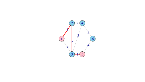
Results of Linear Programming / Linear Optimization

Objective function (Minimum): 4

Iterations in phase 1: 3
Iterations in phase 2: 3
Solution
opt
1 1 1->2
2 0
3 0
4 0
5 1 2->3
6 0
7 0
8 0
9 0
10 0
11 1 3->5
12 0
13 0
14 0
15 0
16 0

Basic Variables
opt
1 1
5 1
11 1
S 1 0
S 5 0
S 6 0

Constraints
actual dir bvec free dual dual.reg
1 1 <= 1 0 0 NA
2 -1 <= -1 0 4 Inf
3 0 <= 0 0 1 Inf
4 0 <= 0 0 3 Inf
5 0 <= 0 0 0 NA
6 0 <= 0 0 0 NA

All Variables (including slack variables)
opt cvec min.c max.c marg marg.reg
1 1 1 -2 2 NA NA
2 0 1 99 77 2 Inf
3 0 5 99 77 2 1
4 0 5 99 77 8 Inf
5 1 2 -5 4 NA NA
6 0 2 99 77 4 Inf
7 0 2 99 77 3 Inf
8 0 2 99 77 1 1
9 0 3 99 77 6 Inf
10 0 3 99 77 0 1
11 1 1 -3 Inf NA NA
12 0 1 99 77 2 Inf
13 0 3 99 77 3 Inf
14 0 3 99 77 3 Inf
15 0 4 99 77 8 Inf
16 0 4 99 77 0 1
S 1 0 0 -1 1 0 NA
S 2 0 0 -4 Inf 4 Inf
S 3 0 0 -1 Inf 1 Inf
S 4 0 0 -3 Inf 3 Inf
S 5 0 0 -3 1 0 NA
S 6 0 0 -3 3 0 NA

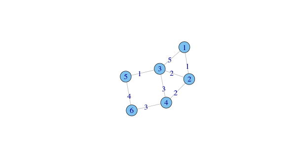
igraphパッケージを使う

library(igraph)
#エッジリストの作成
d <- data.frame(matrix(c( "1","2", "1","3", "2","3", "2","4", "3","4", "3","5", "4","6", "5","6"),nc=2,byrow=TRUE),stringsAsFactors=FALSE)
#ノードリストの作成
vers <- data.frame(c("1","2","3","4","5","6"),stringsAsFactors=FALSE)
#グラフの作成
#無向グラフ(directed=F)
g <- graph.data.frame(d,directed=F,vertices=vers)
#ウエイトの指定
E(g)$weight <- c(1,5,2,2,3,1,3,4)
V(g)$size <-35
plot(g,vertex.label=V(g)$name,edge.label=E(g)$weight)

# p.53のような配置になるように座標を指定する
#ノードの座標の指定
v1<- c(1,2); v2 <- c(2,3); v3 <- c(2,1); v4 <- c(3,3); v5 <- c(3,1); v6 <- c(4,2)
lay <- rbind(v1,v2,v3,v4,v5,v6)
#プロット
plot(g,layout=lay,vertex.label=V(g)$name,edge.label=E(g)$weight)

sum <- get.all.shortest.paths(g, "1", "5", mode="out")
V(g)[sum$res[[1]]]
E(g)$color <- "grey"
E(g, path=sum$res[[1]])$color <- "red" # ※最短経路が複数ある場合は1つ目
E(g, path=sum$res[[1]])$width <- 3
V(g)$color <- "skyblue"   
V(g)$color[1] <- "pink"
V(g)$color[5] <- "pink"
plot(g,layout=lay,vertex.label=V(g)$name,edge.label=E(g)$weight)