回帰分析1

放送大学「心理統計法」第12章　回帰分析

x<-c(10,9,9,8,7,7,6,5,5,4)
y<-c(8,7,6,7,6,6,5,4,3,6)
Model <- lm(y~x)
library(xtable)
print(xtable(Model),type="html")

	Estimate	Std. Error	t value	Pr(>|t|)
(Intercept)	1.9111	1.2452	1.53	0.1634
x	0.5556	0.1717	3.24	0.0120

library(stargazer)
stargazer(Model,type="html",single.row=T,title="線形回帰")

線形回帰

	Dependent variable:
	y
x	0.556 (0.172)
Constant	1.911 (1.245)
Observations	10
R2	0.567
Adjusted R2	0.513
Residual Std. Error	1.030 (df = 8)
F Statistic	10.471 (df = 1; 8)
Note:	p<0.1; p<0.05; p<0.01< td="">

library(texreg)
htmlreg(Model,single.row =T)

Statistical models

	Model 1
(Intercept)	1.91 (1.25)
x	0.56 (0.17)
R2	0.57
Adj. R2	0.51
Num. obs.	10
**p < 0.001, *p < 0.01, p < 0.05

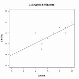
回帰直線を描く

plot(x,y,xlim=c(0,10),ylim=c(0,10),xlab="試験成績",ylab="仕事評価",main="入社試験と仕事評価の関係")
abline(Model,col="red")

線形モデル(切片を0にする)

Model2 <- lm(y~x+ 0)
plot(x,y,xlim=c(0,10),ylim=c(0,10),xlab="試験成績",ylab="仕事評価",main="入社試験と仕事評価の関係")
abline(Model2,col="red")