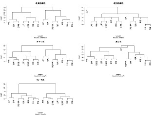
品川<-c(0,7,12,14,18,22,25,28,24,21,17,14,10,7) 目黒<-c(7,0,5,7,11,15,18,23,31,28,24,21,17,14) 渋谷<-c(12,5,0,2,6,10,13,18,22,25,29,26,22,19) 原宿<-c(14,7,2,0,4,8,11,16,20,23,27,28,24,21) 新宿<-c(18,11,6,4,0,4,7,12,16,19,23,26,28,25) 高田馬場<-c(22,15,10,8,4,0,3,8,12,15,19,22,26,29) 池袋<-c(25,18,13,11,7,3,0,5,9,12,16,19,23,26) 巣鴨<-c(28,23,18,16,12,8,5,0,4,7,11,14,18,21) 田端<-c(24,31,22,20,16,12,9,4,0,3,7,10,14,17) 日暮里<-c(21,28,25,23,19,15,12,7,3,0,4,7,11,14) 上野<-c(17,24,29,27,23,19,16,11,7,4,0,3,7,10) 秋葉原<-c(14,21,26,28,26,22,19,14,10,7,3,0,4,7) 東京<-c(10,17,22,24,28,26,23,18,14,11,7,4,0,3) 新橋<-c(7,14,19,21,25,29,26,21,17,14,10,7,3,0) d<-data.frame(品川,目黒,渋谷,原宿,新宿,高田馬場,池袋,巣鴨,田端,日暮里,上野,秋葉原,東京,新橋) row.names(d)<-c("品川","目黒","渋谷","原宿","新宿","高田馬場","池袋","巣鴨","田端","日暮里","上野","秋葉原","東京","新橋") yamate0<-as.matrix(d) yamate1<-as.dist(yamate0) par(mfrow=c(3,2)) yamate4<-hclust(yamate1) plot(yamate4,main="最長距離法") yamate4<-hclust(yamate1,method="single") plot(yamate4,main="最短距離法") yamate4<-hclust(yamate1,method="average") plot(yamate4,main="群平均法") yamate4<-hclust(yamate1,method="centroid") plot(yamate4,main="重心法") yamate4<-hclust(yamate1,method="ward") plot(yamate4,main="ウォード法") par(mfrow=c(1,1))
|